VOLUME 37, ARTICLE 27, PAGES 867
,
888
PUBLISHED 29 SEPTEMBER 2017
http://www.demographic-research.org/Volumes/Vol37/27/ DOI: 10.4054/DemRes.2017.37.27
Research Article
Economic crisis promotes fertility decline in
poor areas: Evidence from Colombia
Eleonora Davalos
Leonardo Fabio Morales
© 2017 Eleonora Davalos & Leonardo Fabio Morales
This open-access work is published under the terms of the Creative Commons Attribution NonCommercial License 2.0 Germany, which permits use, reproduction, and distribution in any medium for noncommercial purposes, provided the original author(s) and source are given credit.
1 Introduction 868
2 Economic crisis and fertility in Colombia 869
3 The economic theory of fertility 873
4 Data 875
4.1 How do poor and well-off states differ? 877
5 Empirical strategy 878
6 Results 879
7 Discussion 882
8 Acknowledgements 883
References 884
Economic crisis promotes fertility decline in poor areas:
Evidence from Colombia
Eleonora Davalos1
Leonardo Fabio Morales2
Abstract
BACKGROUND
The effects of an economic recession extend beyond financial spheres and spill over into present and future family decisions via income restrictions and expectations. Hardly any research on the effects of economic recession on fertility outcomes has taken place in developing countries.
OBJECTIVE
This study seeks to explain the effects of economic cycles on fertility outcomes in poor areas.
METHODS
This paper analyzes fertility trends from the third largest economy in Latin America – Colombia – from 1998 to 2013. We estimate a panel data regression model with state and year fixed effects.
RESULTS
On average, periods of recession are associated with fertility decline in poor areas and fertility growth in well-off areas. During an economic crisis, fertility in poor states decreases by 0.002 children per woman, while in well-off states fertility increases by 0.007 children per woman.
CONCLUSIONS
The impact of an economic crisis on fertility varies depending on poverty. Poor states have procyclical responses while well-off states tend to have countercyclical reactions to economic downturns.
CONTRIBUTION
This study illuminates the procyclical and countercyclical debate, showing that within a country there can be two different responses to an economic downturn.
1. Introduction
A decline in fertility has been perceived as a blessing for developing countries, a reduction in population growth that eases the adversity of poverty and leads to long-lasting development. Known as demographic transition, the long-term decline in the number of children per women has several complementary explanations: the demographic transition theory (Notestein 1953), the theory of wealth flows (Caldwell 1982), the microeconomic theory of fertility (Becker 1960; Schultz 1973), and ideational theory (Cleland and Wilson 1987). Latin America is no exception to this global trend. Most Latin American countries started their demographic transitions around the 1960s, a period in which fertility decline was accompanied by increasing life expectancy, improved literacy rates, and economic growth.
Although economic growth, measured by changes in gross domestic product, has been steadily increasing in the long term, there have been periods in which the economy has decelerated – the late 1970s, mid-1980s, late 1990s, and late 2000s. These periods, in which the economic climate restricted production and consumption, are the focus of this paper. Given that long-term economic growth has been negatively related to fertility, does this mean that short-term setbacks in economic growth have a positive relationship with fertility? There is no single answer: Positive and negative relationships depend on individual characteristics such as age group and education level (Friedman and Levinsohn 2001; Pilkauskas, Currie, and Garfinkel 2012; Ravallion 2010).
Hardly any research on the effects of economic recession on fertility outcomes has taken place in developing countries. Eloundou-Enyegue, Stokes, and Cornwell (2000) find support for a procyclical relationship between economic growth and fertility in Cameroon, and Adsera and Menendez (2011) reach similar conclusions for Latin America. However, neither study addresses the issue that the effects of an economic crisis are contingent on poverty levels (Lustig 2000). An economic crisis will always have a greater impact in poor areas because poor households have less or no savings to face abrupt economic changes (Friedman and Levinsohn 2001; Lustig 2000). Therefore, it can be expected that during periods of economic crisis, poor areas will experience a greater reduction in fertility outcomes than well-off areas. Aiming to fill this gap, this paper analyzes fertility trends in Colombia during the last decades, focusing on one of the most important events that occurred during this period, the economic recession of 1999.
To assess the effect of the economic crisis on fertility outcomes we use annual data on total fertility rates for 32 states and Bogotá, the capital of Colombia, between 1998 and 2013. The concept of poverty is operationalized using the unsatisfied basic needs index (UBN). We estimate a panel data regression model with state and year fixed effects. Our findings suggest that within a country there can be two different responses to a recession because the impact of an economic crisis on fertility varies depending on poverty. In poor areas extreme recession is associated with fertility decline, and in wealthy areas with fertility growth. Therefore, poor states have procyclical responses while well-off states tend to have countercyclical reactions to economic downturns. During an economic crisis, fertility in poor states decreases on average by 0.002 children per woman, while in well-off states fertility increases by 0.007 children per woman.
The paper is organized as follows: Section two documents fertility and economic growth trends in Colombia. Section three presents the theoretical framework used in this analysis. Sections four and five describe the data and analytical strategy used in the econometric analysis. Section six reports the results of the panel data regression, and section seven presents a discussion of the results.
2. Economic crisis and fertility in Colombia
Like most Latin American countries, Colombia started its first demographic transition in the 1960s. Based on World Bank data, in 1960 Colombia had a total fertility rate (TFR) of about 6.8 children per woman.3 This rate fell quite rapidly throughout the 3 Total fertility rate is the average number of children born to a woman if she were to live to the end of her
1960s, 1970s, and 1980s, and started flattening out in the late 1990s at roughly 2.5 children per woman. The solid line in Figure 1 represents the total fertility rate from 1960 to 2014 (left axis). The dashed line shows real (inflation-adjusted) gross domestic product (GDP) per capita over the same period (right axis). GDP per capita has been increasing steadily since 1960 with two periods of slowdown in the 1970s and 1980s and only one major setback, in the late 1990s.4 This paper focuses on this last period of
economic crisis, paying special attention to the consequences of economic recession for fertility outcomes in poor areas.
Figure 1: Total fertility rate and real gross domestic product, Colombia 1960–2014
Notes: Based on World Bank data available at http://data.worldbank.org/indicator
Colombia experienced economic deceleration in 1998, when real GDP grew only 0.6%, and reached its nadir in 1999 with a negative real GDP growth of 4.3%. This economic slowdown rapidly translated into unemployment rate increments of about 4 percentage points, increasing from 12% to 16% (based on data from the National
4 Figure A-1 illustrates the same negative relationship between total fertility rate and GDP per capita using
data from the Demographic Health Surveys available for Colombia.
1000 2000 3000 4000 5000 6000 7000 8000 1 2 3 4 5 6 7
1959 1964 1969 1974 1979 1984 1989 1994 1999 2004 2009 2014
C o n s ta n t 2 0 1 0 U S D C h il d re n p e r w o m a n
Department of Statistics of Colombia). Figure 2 illustrates this trend, showing changes in the annual unemployment rate and TFR 12 months later. The unemployment upturn in 1999 closely matches the fertility downturn in 2000, suggesting that economic hardship could explain, at least in part, changes in the fertility rate.
Figure 2: Changes in unemployment and total fertility rate, Colombia 1998–2013
Notes: Total fertility rates estimated by the authors using data from the Vital Registration System; unemployment rate from the National Department of Statistics. Change in unemployment rate (percentage points) by year and change in total fertility rate (percentage) twelve months later.
An economic recession is traditionally defined as two consecutive quarters of real GDP negative growth (Blanchard 2010; Claessens and Kose 2009). Some of the symptoms of a recession are increased unemployment and reduced consumption. An increase in unemployment rates is likely to increase material hardship, which in turn lowers expectations in future periods (Pilkauskas, Currie, and Garfinkel 2012). Expectations of the future are crucial to present-day decisions, since today’s decisions are based not only on what is happening today but also on the future consequences of those decisions (Bellman 1954). Therefore, poor expectations about the future might deter couples from marrying and having children (Easterlin 1980), because having
-8 -6 -4 -2 0 2 4
1997 1999 2001 2003 2005 2007 2009 2011 2013
children in modern societies is a negative flow of resources that has long-term implications (Caldwell 1982; Morgan, Cumberworth, and Wimer 2011).
The two greatest fertility declines in recent Colombian history occurred at the beginning and the end of the first decade of the 2000s. Between 1999 and 2001, TFR declined by 5%, from 2.2 to 2.1, and between 2008 and 2010 it declined by 7%, from 1.9 to 1.7. Figure 3 shows these fertility declines across different age groups: The total fertility rate (left axis) and age-specific fertility rates (right axis) depict the same story. A macro-level factor that affects fertility decisions in the same way has motivated these changes across different age groups. Most age groups move uniformly until the effect fades for women age 40–44, for whom delaying childbearing is no longer an option.
Figure 3: Total fertility rate and age specific fertility rates, Colombia 1998–2013
Notes: Total fertility rates and age-specific fertility rates estimated by the authors using data from the Vital Registration System. 0 20 40 60 80 100 120 0 0.5 1 1.5 2 2.5
1997 2002 2007 2012
C h il d re n p e r 1 ,0 0 0 W o m e n C h il d re n p e r W o m a n
tfr 15‒119 20‒24
25‒29 30‒34 35‒39
3. The economic theory of fertility
The study of fertility and its relationship to economic and income growth has a history that goes back to the seminal work of Malthus (1967). The modern standard economic modeling of fertility presents fertility outcomes as rational decisions framed in a standard neoclassical model of consumer demand (Becker 1960). In the standard static theoretical framework of fertility, parents derive utility from their children and from a composite good that represents all other consumption (Hotz, Klerman, and Willis 1997). Therefore, parents seek to maximize their utility, subject to a budget constraint that depends on the number of children they have (their consumption of children) and a composite good representing other consumption. In this setting, the budget constraint is a function of prices of the composite good and the price of having children, which includes the opportunity cost of parenting time as well as rearing costs. The result of this optimization process is the demand for children.
Two contributions extend this framework. First, parents get utility from the number of children they have and the quality of child development. Second, the concept of child development is the result of a household production process that depends heavily on parental time (Becker 1960; Mincer 1963; Willis 1973). More recent studies have incorporated dynamics into the study of rational fertility using an overlapping generation (OLG) model. Recent OLG model developments have been used to analyze the role of fertility in models that study the consequences of fertility reduction in pay-as-you-go pension systems (Cipriani 2014; Fanti and Gori 2012). OLG models account for complex intergenerational relationships and are suitable for the study of social security systems, pensions, and demographic change.
The empirical analysis in this study is based on a simple OLG model with endogenous fertility.5 Since our main conclusions derive from our empirical model, we
use a theoretical model to illustrate the intuition of our empirical findings. In our model, an individual lives two periods. When young individuals supply one unit of labor and obtain wages( ), they also decide how much money to save( ) and how many children to have. Old individuals do not work: they spend their savings to pay for consumption. Let us denote the total return on savings as = 1 + , where is the interest rate. We normalize consumption prices to 1 and assume fixed prices of childrearing . We also assume a logarithmic utility function, which is common in the literature on endogenous fertility. The lifetime optimization problem of an individual can be represented as follows:
Equation 1: Optimization problem of an individual
, ( ) + ( ) + ( ) . . = − − ; =
where and stand for a generationt individual’s consumption when young and old andq is the average childrearing cost. Under standard assumptions on the production side of the economy, the solution to this utility maximization problem provides the demand function for children and savings represented in Equation 2.
Equation 2: Demand function for children and savings
= (1 + + ); = (1 + + )
From equations (1) and (2), the optimal number of children in this model is an increasing function of wages, and decreases with higher childrearing costs. Therefore, economic factors can be expected to have an impact on global fertility. Childbearing costs include the opportunity cost of the average parental time required for childrearing. We assume that there is a continuum of the indexes of household type by ∈ [0,1], and wages and childrearing cost are continuous functions of this index.6 We can then find
how variation in wages and childrearing costs affects fertility when increases using the total change of . Assuming that represents household heterogeneity, this total derivative can be represented as:
Equation 3: Variation in wages and childrearing costs
= ∙ + ∙ ≈ (1 + + )∆∆ − (1 + + )∆∆
Note that we are assuming that wages are implicit functions of the continuous index .7 The previous equations describe this situation for a heterogeneous household.
Fertility changes, given changes in household skills, are ambiguous and depend on the sensitivity of wages and childrearing costs to the index , which represents the household ‘quality.’ In a state with richer households on average, the childrearing cost (including opportunity cost) will be substantially higher than in other states. Given our
6 This is just a simple way to illustrate the idea that more skilled (or wealthy) individuals have better wages
and spend more on rearing their children.
7 An intuitive assumption is that wages and childrearing costs are convex functions of , since labor income
assumptions, the term∆
∆ in equation (3) will be large. In this case, the second term of the previous expression may be higher in magnitude that the first term, and the whole expression will be negative. Analogously, in poor states the opportunity cost, and in general the cost of childbearing, will be lower than in other states. The term∆
∆ in equation (3) will be small, and the whole expression will turn positive.
Finding the marginal changes in equation (3), given changes in wages, reveals how macroeconomic shocks impact the fertility rate because economic booms and recessions effect wages. Assuming that economic booms (recessions) increase (decrease) average wages and the relative wage gap between rich and poor states remains constant or increase in favor of rich states, the final response on fertility will depend on the relative wealth of individuals and states. Under our assumptions, a possible prediction of this model is that the effect of economic booms (recessions) will be negative (positive) in rich states and positive (negative) in poor states.
Malthus (1967) and others predicted a positive relationship between fertility and wages. This conclusion was widely supported in the subsequent literature (Felderer 1990; Raut 1990). There is a very interesting result in Becker, Murphy, and Tamura (1990), which can be easily applied to developing economies. This paper finds that in cases where per capita income is very low, to the extent that childrearing costs are a substantial part of it, the relation between fertility and wages is positive (Zhang and Zhang 1997). Some general results contradict this. The most influential, from Barro and Becker (1989), imply a negative relationship between wages and fertility. In the context of overlapping generation models, Zhang and Zhang (1997) reconcile the evidence by suggesting both positive and negative effects of wages on fertility. Using different options for utility functions, they show that fertility and wages are positively correlated when bequests are non-operative.
4. Data
This paper uses birth data from the Colombian vital registration system to produce total fertility rate (TFR) and age-specific fertility rate (ASFR) estimates for 32 states and Bogotá, the Colombian capital. The analyzed period covers 16 years, from 1998, the year in which the National Department of Statistic of Colombia started collecting birth certificate data, to 2013, producing a dataset of TFR and ASFR for each state during this time span.
analysis the concept of economic crisis is equivalent to real GDP growth.8 To classify
states by wealth we use unsatisfied basic needs (UBN) from the National Planning Department. This measure ranges from zero to a hundred depending on the percentage of households with one or more unsatisfied basic needs: higher UBN values indicate the presence of more households with unsatisfied needs. This indicator captures four different factors associated with poverty: inadequate housing materials (e.g., paper, wood, cement), inadequate access to running water and sewage, overcrowding, school-age children not enrolled in school, and economic dependence. Based on annual state-level UBN measures, we classify states into two groups: ‘poor’ states and ‘well-off’ states. States in which the percentage of households with a UBN above the country’s UBN level are considered poor, while states with a UBN below the country’s UBN level are considered well off. By classifying states into poor and well off, we aim to distinguish the effect of the economic crisis on poor states from its effect on well-off states.
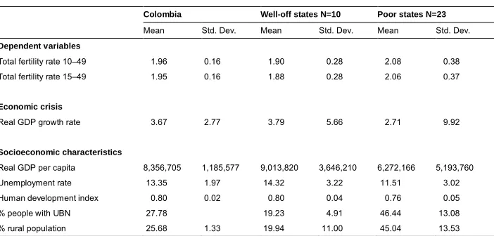
The analysis also includes main covariates to control for other state-level characteristics. We use the Human Development Index (HDI) from the United Nations Development Program to measure human development. This index combines indicators of life expectancy, educational attainment, and income in a single measure that ranges from zero to one, in which values closer to one represent more social and economic development. We also control for unemployment rate, the percentage of rural population, and average income calculated using real GDP and total population in each state, all these variables from the National Department of Statistics of Colombia. Means and standard deviations of these variables may be found in Table 1. The final dataset consists of 33 cross-sectional units – 32 states and the capital – along a time span of 16 years (1998–2013), creating a balanced panel.
Table 1: Descriptive statistics variables included in panel data regressions, Colombia 1998–2013
Colombia Well-off states N=10 Poor states N=23
Mean Std. Dev. Mean Std. Dev. Mean Std. Dev.
Dependent variables
Total fertility rate 10–49 1.96 0.16 1.90 0.28 2.08 0.38
Total fertility rate 15–49 1.95 0.16 1.88 0.28 2.06 0.37
Economic crisis
Real GDP growth rate 3.67 2.77 3.79 5.66 2.71 9.92
Socioeconomic characteristics
Real GDP per capita 8,356,705 1,185,577 9,013,820 3,646,210 6,272,166 5,193,760
Unemployment rate 13.35 1.97 14.32 3.22 11.51 3.02
Human development index 0.80 0.02 0.80 0.04 0.76 0.05
% people with UBN 27.78 19.23 4.91 46.44 13.08
% rural population 25.68 1.33 19.94 11.00 45.04 13.53
Notes: Total fertility rates estimated by the authors using data from the Vital Registration System. GDP growth, GDP per capita, unemployment rate, and rural population from the National Department of Statistics. Human Development Index from the United Nations Development Program.
4.1 How do poor and well-off states differ?
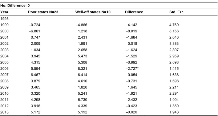
On the one hand, in terms of real GDP growth rate, poor and well-off states are very alike. During the period of study, on average, GDP growth was 2.71 in poor states and 3.71 in well-off states. Comparing annual GDP growth for both groups supports the same observation and provides additional insights. Throughout the 15 years of the period of study there is no statistically significant difference between GDP growth in poor and well-off states. Table 2 summarizes the results of a group mean test for each year. GDP growth in poor and well-off states differs significantly in only one year, 2006, a bonanza year when Colombian GDP growth reached 6.7%.
On the other hand, on average the percentage of households with unsatisfied basic needs in poor states is more than twice that in well-off states. The percentage of rural population in poor states is almost double that in well-off states, and the unemployment rate is lower.9 In addition, well-off states have a high level of human development (HDI
greater than 0.75), whereas poor states have a medium level (HDI greater than 0.64). Therefore all these factors are included as control variables in the analysis.
9 Potential explanations of the lower unemployment rates in poor states include self-employment in
Table 2: Group mean test for real annual GDP growth
Ho: Difference=0
Year Poor states N=23 Well-off states N=10 Difference Std. Err.
1998
1999 –0.724 –4.866 4.142 4.769
2000 –6.801 1.218 –8.019 8.156
2001 0.747 2.431 –1.684 2.646
2002 2.009 1.991 0.018 3.383
2003 1.034 2.658 –1.624 2.897
2004 3.945 5.473 –1.529 2.959
2005 4.315 5.308 –0.992 2.098
2006 5.594 8.321 –2.727* 1.415
2007 6.467 6.414 0.054 1.638
2008 3.879 4.610 –0.731 1.698
2009 3.465 1.820 1.645 2.211
2010 3.320 5.241 –1.921 2.291
2011 4.298 6.730 –2.432 1.994
2012 3.916 4.339 –0.423 1.350
2013 5.172 5.192 –0.020 1.943
Notes: * p<0.10
5. Empirical strategy
To assess the effect of the economic crisis on fertility outcomes, we estimate a panel data regression model with state and year fixed effects. This approach controls for unobservable cross-state differences: for instance, cultural attitudes towards the use of contraception. The model is estimated using Huber–White standard errors, clustered by state to control for arbitrary correlation within a state. The basic econometric model is presented in Equation 4.
Equation 4: Panel data model assessing the effect of the economic crisis on fertility outcomes in poor areas
= + + + + ′ + + +
where = 1, … ,33, and = 1, … , 16.
The outcome variable is the total fertility rate in state and year . is a dichotomous variable that takes the value of one if the state is poor and zero otherwise for state and year . is a continuous variable measuring economic growth.
measures the average change in the total fertility rate as a result of changes in the economic environment given the type of state. is a vector of control variables that includes unemployment rate, percentage of rural population, human development, and a time trend to control for the effect of time on fertility decline. The model also includes state fixed effects( ) to capture time-invariant state-specific characteristics that may confound the estimate of interest, and time fixed effects ( ) to control for variables that are constant across states but evolve over time. The term is a stochastic error term.
6. Results
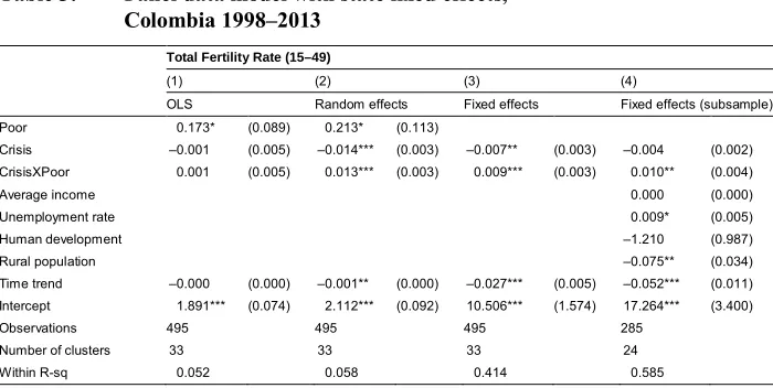
Fertility in Colombia, as in many other developing countries, follows a long-term decline that is the product of a combination of increasing education, declining mortality rates, and economic growth (Bongaarts and Watkins 1996). In other words, fertility decline is the result of improvements in the standard of living. This is true both at the country level and for states. Table 3 illustrates this long-term tendency, as the time trend is always negative and statistically significant. This table presents three specifications with fairly similar results across columns. Models (1) and (2) address the association between economic cycles and fertility decline by pooled ordinary least squares (Pooled OLS) and random effects. Models (3) and (4) analyze the same relationship by fixed effects. Numbers in parentheses are Huber–White standard errors clustered by state.
Results from models (1) and (2) are base line specifications. Pooled OLS estimators are biased and inconsistent because omitted unobservable cross-state differences are potentially correlated with the other regressors. Random effects estimators are presented to illustrate the differences between random and fixed effect methodology. In this case, the Hausman test favors fixed-effects estimations over random-effects estimations. Therefore, models (3) and (4) are the results of interest.
Table 3: Panel data model with state fixed effects, Colombia 1998–2013
Total Fertility Rate (15–49)
(1) (2) (3) (4)
OLS Random effects Fixed effects Fixed effects (subsample)
Poor 0.173* (0.089) 0.213* (0.113)
Crisis –0.001 (0.005) –0.014*** (0.003) –0.007** (0.003) –0.004 (0.002) CrisisXPoor 0.001 (0.005) 0.013*** (0.003) 0.009*** (0.003) 0.010** (0.004)
Average income 0.000 (0.000)
Unemployment rate 0.009* (0.005)
Human development –1.210 (0.987)
Rural population –0.075** (0.034)
Time trend –0.000 (0.000) –0.001** (0.000) –0.027*** (0.005) –0.052*** (0.011) Intercept 1.891*** (0.074) 2.112*** (0.092) 10.506*** (1.574) 17.264*** (3.400)
Observations 495 495 495 285
Number of clusters 33 33 33 24
Within R-sq 0.052 0.058 0.414 0.585
Notes: This table presents the results of the specification established in equation 4 by panel data regression. The outcome variable used in this analysis is total fertility rate (15–49). The sample comprises 32 states and Bogotá, the capital, between 1998 and 2013. Year and state fixed effects regressors in model (3) and (4) not shown. Huber–White standard errors clustered by state in parentheses. *** p<0.01, ** p<0.05, * p<0.10
Poor states, by contrast, respond in the opposite direction to reductions in GDP growth. If during the period of study there is an economic contraction – GDP growth decreases by one percentage point – the total fertility rate in poor states decreases on average by 0.002 (0.009–0.007) children per woman. Results from model (4), including additional control variables,10 are consistent with the results from model (3). If GDP
growth decreases by one percentage point during the period of study, the total fertility rate in poor states decreases on average by 0.006 (0.010–0.004) children per woman. Table 4 presents the marginal effects of economic crisis on the total fertility rate for model (3). This table illustrates how the effect of economic crisis on the fertility rate is moderated by poverty. Worsening economic conditions are associated with fertility growth in well-off states and fertility decline in poor states. Figure 4 illustrates these marginal effects.
10 Sample reduction due to data availability, state-level UBN is available for only 23 states and the capital
Table 4: Marginal effects of economic crisis, model (3)
Marginal effect Moderator Coefficient Std. Err.
Crisis Poor 0 –0.007** 0.001
1 0.002* 0.003
Notes: This table presents the marginal effects of economic crisis based on the results of model (3). ** p<0.05, * p<0.10
Figure 4: Effects of economic crisis on fertility outcomes moderated by poverty level, Colombia 1998–2013
Notes: Based on table 3 and 4, model (3). Error bars 90% confidence intervals.
Coefficients on poverty from models (3) and (4) are not reported in Table 3 because the percentage of people with unsatisfied basic needs varies from one year to another, but when the index is compared with the national level the relationship is constant. Therefore, states remain constantly poor or well off throughout the period of study. As a consequence, state fixed effects capture this time invariant effect.
-0.014 -0.012 -0.010 -0.008 -0.006 -0.004 -0.002 0.000 0.002 0.004
1
C
h
a
n
g
e
T
F
R
7. Discussion
An economic crisis is a macro-level shock that affects everyone. Nevertheless, the consequences of an economic recession can be diverse depending on age group, sex, and level of education (Friedman and Levinsohn 2001; Pilkauskas, Currie, and Garfinkel 2012; Ravallion 2010). The main findings of this macro-level analysis suggest that poor and wealthy areas respond differently to periods of economic hardship. In terms of fertility outcomes, poor states have procyclical responses to economic downturns while well-off states tend to have countercyclical reactions. On average, periods of recession are associated with fertility decline in poor areas and fertility growth in well-off areas. This is not to say that economic crisis is the only factor affecting fertility outcomes, but rather that it promotes fertility decline in poor areas.
When interpreting these results, there are some operational limitations to consider. First, this aggregate period analysis uses composite indexes to control for life expectancy, educational attainment, income, inadequate housing, inadequate access to running water and sewage, overcrowding, school-age children not enrolled in school, and economic dependence; all indicators associated with poverty. However, because of the aggregate nature of the indexes it is impossible to isolate the exact effect of each of these factors on fertility outcomes. In addition, temporal differences in TFR between poor and wealthy areas might suggest that abrupt economic changes lead to tempo effects. However, the delimitation of the short-run tempo effect from the long-run quantum effect is beyond the scope of this study and remains material for future research.
8. Acknowledgements
References
Adsera, A. and Menendez, A. (2011). Fertility changes in Latin America in periods of economic uncertainty. Population Studies 65(1): 37–56.doi:10.1080/00324728. 2010.530291.
Barro, R.J. and Becker, G.S. (1989). Fertility choice in a model of economic growth.
Econometrica 57(2): 481–501.doi:10.2307/1912563.
Becker, G.S. (1960). An economic analysis of fertility. In: Roberts, G.B. (ed.).
Demographic and economic change in developed countries. Princeton: Princeton
University Press: 209–231.
Becker, G.S., Murphy, K.M., and Tamura, R. (1990). Human capital, fertility, and economic growth. Journal of Political Economy 98(5): S12–S37. doi:10.3386/ w3414.
Bellman, R. (1954). Decision making in the face of uncertainty–I. Naval Research Logistics Quarterly 1(3): 230–232.doi:10.1002/nav.3800010311.
Blanchard, O. (2010).Macroeconomics. Upper Saddle River: Pearson Prentice Hall. Bongaarts, J. (1978). A framework for analyzing the proximate determinants of fertility.
Population and Development Review 4(1): 105–132.doi:10.2307/1972149.
Bongaarts, J. and Watkins, S.C. (1996). Social interactions and contemporary fertility transitions. Population and Development Review 22(4): 639–682.doi:10.2307/ 2137804.
Butz, W.P. and Ward, M.P. (1979). Will US fertility remain low? A new economic interpretation.Population and Development Review 5(4): 663–688.doi:10.2307/ 1971976.
Caldwell, J.C. (1982).Theory of fertility decline. London: Academic Press.
Cipriani, G. (2014). Population aging and PAYG pensions in the OLG model.Journal
of Population Economics 27(1): 251–256.doi:10.1007/s00148-013-0465-9.
Claessens, S. and Kose, M.A. (2009). What is a recession?Finance and Development
46(1): 52.
Easterlin, R.A. (1980). Birth and fortune: The impact of numbers on personal welfare. New York: Basic Books.
Eloundou-Enyegue, P.M., Stokes, C.S., and Cornwell, G.T. (2000). Are there crisis-led fertility declines? Evidence from central Cameroon. Population Research and
Policy Review 19(1): 47–72.doi:10.1023/A:1006423527473.
Fanti, L. and Gori, L. (2012). Fertility and PAYG pensions in the Overlapping Generations Model. Journal of Population Economics 25(3): 955–961.
doi:10.1007/s00148-011-0359-7.
Felderer, B. (1990). Neoclassical growth with microfoundations.Journal of Economics:
Zeitschriften für Nationalökonomie 51(3): 273–285.doi:10.1007/BF01227425.
Friedman, J. and Levinsohn, J. (2001). The distributional impacts of Indonesia’s financial crisis on household welfare: A ‘Rapid Response’ methodology. Cambridge: National Bureau of Economic Research (NBER Working Paper No. 8564).doi:10.3386/w8564.
Galbraith, V.L. and Thomas, D.S. (1941). Birth rates and the Interwar Business Cycles.
Journal of the American Statistical Association 36(216): 465–476.doi:10.1080/ 01621459.1941.10500587.
Hotz, J., Klerman, J.A., and Willis, R.J. (1997). The economics of fertility in developed countries. In: Rosenzweig, M.R. and Stark, O. (eds.). Handbook of Population
and Family Economics. Amsterdam: Elsevier: 275–347.
doi:10.1016/S1574-003X(97)80024-4.
Lee, R. (1990). The demographic response to economic crisis in historical and contemporary populations.Population Bulletin Of The United Nations29: 1–15. Lustig, N. (2000). Crises and the poor: Socially responsible macroeconomics.
Economia: Journal of the Latin American and Caribbean Economic Association
1(1): 1–19.
Malthus, T.R. (1967).An essay on the principle of population. London: Dutton.
Miller, G., and Urdinola, B.P. (2010). Cyclicality, mortality, and the value of time: The case of coffee price fluctuations and child survival in Colombia. Journal of
Political Economy118(1): 113–155.doi:10.1086/651673.
Mincer, J. (1963). Market prices, opportunity costs, and income effects. In: Christ, C.F. (ed.). Measurement in economics: Studies in mathematical economics and
econometrics in memory of Yehuda Grunfeld. Stanford: Stanford University
Morgan, S.P., Cumberworth, E., and Wimer, C. (2011). The Great Recession’s influence on fertility, marriage, divorce, and cohabitation. In: Grusky, D.B., Western, B., and Wimer, C. (eds.). The Great Recession. New York: Russell Sage Foundation: 220–245.
Neels, K., Theunynck, Z., and Wood, J. (2013). Economic recession and first births in Europe: Recession-induced postponement and recuperation of fertility in 14 European countries between 1970 and 2005. International Journal Of Public
Health 58(1): 43–55.doi:10.1007/s00038-012-0390-9.
Notestein, F.W. (1953). Economic problems of population change. London: Oxford University Press.
Pilkauskas, N.V., Currie, J.M., and Garfinkel, I. (2012). The Great Recession, public transfers, and material hardship. Social Service Review 86(3): 401–427.
doi:10.1086/667993.
Raut, L.K. (1990). Capital accumulation, income distribution and endogenous fertility in an Overlapping Generations General Equilibrium Model. Journal of
Development Economics 34: 123–150.doi:10.1016/0304-3878(90)90079-Q.
Ravallion, M. (2010). The developing world’s bulging (but vulnerable) middle class.
World Development 38(4): 445–454.doi:10.1016/j.worlddev.2009.11.007.
Rindfuss, R., Morgan, S.P., and Swicegood, G. (1988). First births in America: Changes in the timing of parenthood. Berkeley: University of California Press. Santow, G. and Bracher, M. (2001). Deferment of the first birth and fluctuating fertility
in Sweden. European Journal of Population 17(4): 343–363. doi:10.1023/ A:1012527623350.
Schultz, T.W. (1973). New economic approaches to fertility. Proceedings of a conference, June 8–9, 1972. Chicago: University of Chicago Press.
Silver, M. (1965). Births, marriages, and business cycles in the United States.Journal of Political Economy73(3): 237.doi:10.1086/259013.
Sobotka, T., Skirbekk, V., and Philipov, D. (2011). Economic recession and fertility in the developed world. Population and Development Review 37(2): 267–306.
doi:10.1111/j.1728-4457.2011.00411.x.
Willis, R.J. (1973). A new approach to the economic theory of fertility behavior.
Appendix
Figure A-1: Total fertility rate and real gross domestic product, Colombia 1986–2010
Note: Total fertility rate data from DHS in Colombia. GDP per capita data from World Bank.
3500 4000 4500 5000 5500 6000 6500
2 2.2 2.4 2.6 2.8 3 3.2 3.4 3.6
1986 1990 1995 2000 2005 2010
C
o
n
s
ta
n
t
2
0
1
0
U
S
D