Development of ANN Model for Prediction of Coating
Thickness in Hot Dip Galvanizing Process
Sanjeev Kumar Shukla
1*, Anup Kumar Sadhukhan
2, Parthapratim Gupta
21 Steel Products Group, Research and Development Centre for Iron Steel, Steel Authority of India, Ranchi-834002, India.
2 Chemical Engineering Department, National Institute of Technology, Durgapur-713209, India.
* Corresponding author: Tel.: +91-8986889279; email: [email protected] Manuscript submitted October 21, 2016; accepted February 4, 2017.
doi: 10.17706/ijmse.2017.5.2.60-68
Abstract: Hot dip galvanizing of steel strip is carried out in Continuous Galvanizing Lines (CGL) in order to achieve consistency in thickness & quality of Zn-coating. The process is a complex one and is always in dynamic equilibrium depending on various process parameters. Around 20 process parameters, grouped into major sections like steel strip characteristics, pre-treatment, galvanizing process conditions, bath conditions, post treatment operations, are involved in the process. Zn-coating thickness is a nonlinear and coupled function of most of the above process input parameters. In the present work Artificial Neural Network (ANN) has been used to develop an off-line model to predict the coating thickness. Six factors that were identified through sensitivity analysis based on Taguchi’s Orthogonal Array Technique were used as independent variables in the ANN model. A Hot Dip Process Simulator (HDPS) was used to generate the input-output data with close control of input process parameters.The data set generated for training purpose has the coating thickness variation between 12 to 32 µm. The model, developed with total data-sets (234), has the prediction error of 10%. However, the maximum sets (183) lie in the range of 20-30 µm and model developed by taking these data-sets in this range has the prediction error of 7%. In both the cases a 6-(9-6-3)-1 network structure was used & 3/4 of data-sets were used for training & testing & 1/4 for validation.
Keywords: Galvanizing process, coating thickness, artificial neural network, predictive model.
1.
Introduction
importance of controlling the coating thickness & its uniformity for quality & cost of galvanized sheet has been well established [1]-[6].
During the last few decades, model based process control in CGL has been reported by many researchers [7]-[15]. Some of the models have been developed through experimentation in simulator. As the conventional Regression Analysis (RA) is not suitable to assess the effect of such non-linear & interacting process input-output relationship, Artificial Neural Network (ANN) was chosen as the tool to develop a Predictive Mathematical Model. The concepts & application of Artificial Neural Network (ANN) based process control for galvanizing and other manufacturing processes have been described elsewhere [16]-[24].
Presently, on-line model based control of Air-knife wiping system for control of coating thickness & its uniformity uses any three or four of the following process variables as inputs:
i) Strip to knife distance (mm) ii) Strip speed (m/min)
iii) Wiping gas pressure at nozzle (mbar) iv) Nozzle opening (mm)
This article describes the process and outcome of the development of an off-line ANN model to predict the coating thickness based on six process input parameters/factors. Hot Dip Process Simulator (HDPS), a laboratory-scale experimental set-up to study the actual galvanizing process, was used for experimentations and data generation. An ANN model was developed, trained and validated by the experimental data.
2.
Mathematical
Model
2.1.
Modeling for Galvanizing Process
The Zn-coating thickness depends on the chemical kinetics associated with transport limitations. Linares proposed the first mathematical model, which depicted the diffusion phenomena for iron and aluminium in the bath. The growth of the interfacial alloy was assumed to be controlled by iron diffusion through this alloy. Tang [10] assumed that the growth of the interfacial alloy layer was controlled by aluminium diffusion in the bath. He proposed a model for nucleation and growth of the alloy layer. Giorgi et al [24] developed a model to predict the concentration profile of iron and aluminium as a function of galvanizing time and the time needed to form a continuous layer. However, the phenomenological models developed so far are inadequate to incorporate all the hysic-chemical processes involved in galvanizing.
2.2.
Artificial Neural Network (ANN)
In recent times Artificial Neural Network (ANN) is being effectively used in various fields of engineering and science. In the field of multivariate modeling ANN offers many advantages over conventional multiple linear regression methods. Artificial neural networks can identify patterns between the dependent and independent variables in data sets. Furthermore, they can create a specialized regression model or model adjustment for all patterns discovered during analysis.
3.
Experimental
3.1.
Experimentation in HDPS
In HDPS one can change the settings of various inputs under study from one experiment to another. After conducting a matrix experiment, the data from all experiments in the set were taken together and analyzed to determine the effects of different inputs. Zn–coating was made over 200mm x 120mm Cold Rolled sheet samples with thickness of around 0.5 mm in an HDPS in accordance with the Design of Experiments (DoE). The sheet samples were annealed and dipped in the molten Zinc–bath (~35 kg weight).
After galvanizing the coating thickness of all the experimental samples were measured by a magnetic type portable Coating Thickness Gauge (Make: Defalsko, Model: Positector 6000). The thickness of each side of the coated samples was worked out on the basis of 9 measurements covering about 80mm x 80mm area of the central region. The mean of the thickness of both the sides was considered as the coating thickness of one experimental sample. Hence, the coating thickness of each experiment is actually the mean of 18 measurements. Different baths were prepared to vary the Al content of the bath. One experiment was carried out for each set of parameters. DoE was planned such that maximum variations and combination of inputs are possible keeping the number of experiments low. The experiments were conducted in two phases.
3.2.
Sensitivity Analysis
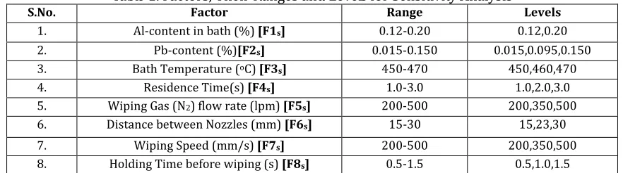
A sensitivity analysis was carried out to identify the critical variables. Design of experiments was formulated using Taguchi’s Orthogonal Array Technique and encompassing the entire range of actual operation of a CGL with 8 process parameters as factors. From Taguchi’s Orthogonal Array Selector the corresponding orthogonal array is found to be L18. The ranges and the levels of the 8 factors at which the experiments were carried out in HDPS to generate the data for the sensitivity analysis are presented in Table 1.
Table 1. Factors, Their Ranges and Levels for Sensitivity Analysis
S.No. Factor Range Levels
1. Al-content in bath (%) [F1s] 0.12-0.20 0.12,0.20
2. Pb-content (%)[F2s] 0.015-0.150 0.015,0.095,0.150
3. Bath Temperature (oC) [F3s] 450-470 450,460,470
4. Residence Time(s) [F4s] 1.0-3.0 1.0,2.0,3.0
5. Wiping Gas (N2) flow rate (lpm) [F5s] 200-500 200,350,500
6. Distance between Nozzles (mm) [F6s] 15-30 15,23,30
7. Wiping Speed (mm/s) [F7s] 200-500 200,350,500
8. Holding Time before wiping (s) [F8s] 0.5-1.5 0.5,1.0,1.5
Out of 8 factors Pb-content in bath & wiping speed were discarded and the following six dominant factors were identified for inclusion in the development of the predictive model for coating mass/thickness.
Al-content in bath (%) [F1]
Bath Temperature (oC) [F2]
4.
Development of ANN Model
4.1.
Training of ANN
The ranges and the levels of the 6 factors at which the experiments were carried out in HDPS to generate the training data are presented in Table 2.
Table 2. Factors, Their Ranges and Levels for Training the ANN Model
S.
No Factor Range Levels
1. Al-content in bath (%) [F1] 0.10-0.28 0.10, 0.12, 0.14, 0.16, 0.18,
0.20, 0.22, 0 .24, 0.26, 0.28
2. Bath Temperature (oC) [F2] 445-470 445, 450, 455, 460, 465, 470
3. Distance between Nozzles (mm) [F3] 15-17 15, 16, 17
4. Holding Time before wiping (s) [F4] 0.1-2.1 0.1, 1.1, 2.1
5. Residence Time(s) [F5] 1.5-3.5 1.5, 2.5, 3.5
6. Wiping Gas (N2) flow rate (lpm) [F6] 200-450 200, 250, 300, 350, 400, 450
Scaling and de-scaling of input and output data were carried out for efficient network training. In the present work batch-mode training was employed where weights were updated after each epoch for all the samples in the training data set. The error between neural network prediction from the input set used for training and target output was fed back to the neural network to update the internal weights and biases of the neural network. The back propagation training rule was used to adjust the weight and bias vectors of network in order to achieve the desired goal for sum-squared error of the network. The final values for weights and biases are the design values for the network and were used to predict the system performance variable. `
4.2.
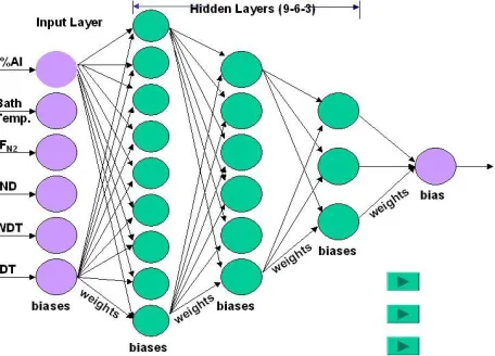
The Network Architecture
A Multi Layer Feed Forward (MLFF) network was selected in the present work. After a large number of trials it was finally decided to have one input layer and three hidden layers and one output layer. Input layer contains six neurons (six factors), 1st hidden layer contains 9, 2nd hidden layer contains 6 neurons, 3rd hidden layer contains 3
Amultiple input-single output relation mapped by an ANNwith one hidden layer can be expressed as:
2
.(
2. ( .
1 1 1)
2)
y F w F w x b
b
(1)where
x
is the input vector, Wi, and Bi, are connection weight and bias matrices, respectively, yis the output vector, and Fiis an activation function, which may be thought of as providing a nonlinear gain for the artificial neuron. Keeping in mind the nonlinear nature of the process, sigmoid functions were chosen for three hidden layers and linear function for final output layer.F(
x
) = 2/[1+exp(-2x
)]-1 (2)The convergence criterion is chosen as mean of sum of the square of the errors for all the experimental findings as 0.018. The configuration of network described above has 6 × 8 no of weights and 8 numbers of biases in the first hidden layer, 8 × 6 weights and 6 biases in the second hidden layer and 6 × 3 weights and 3 biases in the third hidden layer. For output layer there are 3 × 1 numbers of weights and 1 bias. Around 2,000 iterations were required to achieve the desired goal of error level.
The entire operation starting from network architecture, error calculation and training of the network was carried out using Neural Network toolbox of MATLAB. A general purpose MATLAB command line program was developed to use the different functions of the neural network toolbox. The following functions were used.
4.3.
Training Algorithm
The salient steps are presented below. Steps of Gradient Based Training Algorithms : Step 1: Initial guess k = 1
Step 2: If (ETr (k) < e (given accuracy criteria) or k > kmax (max number of iterations).
Step 3: CalculateETr and ETr
w
using partial or all training Data.
Step 4: Use optimization algorithm to find w. Step 5: Update weights as w=w+w.
Step 6: If all training data are used, then k =k+1, go to Step 2, else go to Step 3. Scaled conjugate gradient method was used in the present work.
The expressions for different errors are shown below.
1/
1 max min
(
, )
1
( )
(
).
q q mj k jk
Tr
k Tr j j j
p x w
t
E
w
size Tr m
p
p
(3) 1/1 max min
(
, )
1
( )
(
).
q q mj k jk
Te
k Te j j j
p x w
t
E
w
size Te m
p
p
x: input of the original modeling problem or the neural network. p: predicted output of the neural network.
w: internal weights/parameters of the neural network. m: number of outputs of the model.
t: target data for input set. q: generally 2.
4.4.
Data Analysis & Filtering
All the experimental data were analyzed & filtered with respect to the following:
i) The mean & the maximum of the standard deviation values of the coating thickness ii) The difference between the mean coating thickness values at the two sides
iii) The effects of individual parameters on the coating thickness 234 data sets (after filtering) were considered for model development.
4.5.
Training & Validation of Neural Network
Witten & Frank [25] and Swingler [17] proposed that one-third of the data be withheld for validation and the remaining two-thirds be used for training and testing. Using this approach to avoid the phenomenon of over-training, all the 234 experimental data sets were sorted in increasing order of coating thickness. Then half of the data sets were used for training; one-fourth for validation and the remaining one-fourth was marked as test set. Training set, Test set and Validation set followed the order 1, 3, 5, …. ; 2, 6,10, …& 4, 8, 12, … respectively.
5.
Results and Discussion
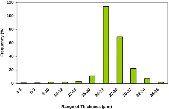
The validation set and test set were fed to the network during training session and the network not only calculated the training error but also the error for validation and test set. The network weights and biases were updated based on training error. With continuous updating of weights and biases training error reduced continuously, while the test and validation error might remain constant or increase with updating. At this point the training was stopped though the error of training set does not reach the desired level. This methodology is called early stopping of network during training phase. The frequency distribution of the data (Fig. 2) shows that most of the data lie in the range 12-32 m.
0 20 40 60 80 100 120
4-5 5-9 9-10 10-1
2 12-1
5 15-2
0 20-2
7 27-3
0 30-3
2 32-3
4 34-3
6
F
re
q
u
e
n
c
y
(
%
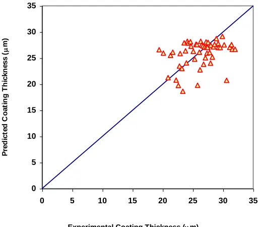
As ANN model needs a large number of data for proper training and validation, this range with 219 data was selected for final model development. The comparison between model predicted & actual values and the mean validation error (0.130) are depicted in Fig. 3 and Fig. 4.
-0.40 -0.20 0.00 0.20 0.40
0 10 20 30 40 50
Experiment No
R
e
la
ti
v
e
E
rr
or
Fig. 3. Relative error between experimental and predicted coating thickness.
0 5 10 15 20 25 30 35
0 5 10 15 20 25 30 35
Experimental Coating Thickness (m)
P
re
d
ic
te
d
C
oa
ti
n
g
T
h
ic
k
n
e
s
s
(
m)
Fig. 4. Comparison between experimental and predicted coating thickness.
The relative errors for model training & validation are depicted in Table 3.
Table 3. Relative Errors for Model Training & Validation
Based on Range Data selected / Total Data Training Error Validation Error
Actual thickness 12-32 219/234 0.110 0.130
Maximum thickness 12-32 219/234 0.072 0.081
error arising out at lower values, the mean training & validation errors decreased to 0.072 and 0.081 respectively (Table 3).
6.
Conclusions
The following conclusions may be made from the outcome of this work:
1) An ANN model has been developed to predict the coating thickness in a hot dip galvanizing process. Multilayered feed-forward network with a 6-(9-6-3)-1 architecture is found suitable for the model.The ANN model developed is found to be effective in predicting the galvanizing coating thickness.
2) As the thickness data was scattered over a wide range and there was a reasonable concentration of data in the range of 12-32 m, such data range was selected for model training and validation. The relative errors of the model for the thickness range of 12-32 µm with a reasonable concentration of data in training and validation were 0.110 and 0.130 respectively based on actual thickness and were 0.072 and 0.081 respectively based on maximum thickness.
References
[1] Butler, J. J., Beam, D. J., & Hawkins, J. C. (1970). The development of air coating control for continuous strip galvanizing. Iron & Steel Engineer, 47(2), 77- 86.
[2] Oren, E. C., Ptashnik, W. S., & Martin, D.C. Galvatech’95 Conference Proceedings (pp. 67-73). [3] Davene, L. Dondin, J.K. Kim & S.J. Kim. Galvatech’95 Conference Proceedings (pp. 205-213).
[4] Dubois, M., Riethmuller, M. L., Buchlin, J. M., & Arnalsteen, M. Galvatech’95 Conference Proceedings (pp. 667-673)
[5] Caignard, S., & Dubois, M. Gatvatech’04 Conference Proceedings (pp. 207-216).
[6] Deote, A. P., Gupta, M. M., Zanwar, D. R. (2012). Process parameter optimization for zinc coating weight control in continuous galvanizing line. International Journal of Scientific & Engineering Research, 3(11), 1-6. [7] Liberski, P., Tatarek, A., & Mendala, J. (2013). Investigation of the initial stage of hot dip zinc coatings on iron
alloys with various silicon contents. Solid State Phenomena., 212, 121–126. [8] Blohm, H. Intergalva’79 (pp. 215-218). London: Zinc Development Association.
[9] Townsend, C. S., & Bilski, W. C. (1988). Closed-loop control of coating weight on a hot dip galvanizing line. Iron & Steel Engineer, 65(7), 44-47.
[10]Tang, N. Y. (1995). Modeling Al enrichment in galvanized coatings. Metallurgical and Materials Trans. A, 26(7), 1699-1704.
[11]Chakkingal, U., & Wright, R. N., Galvatech’95 Conference Proceedings (pp. 823-829).
[12]Laviosa, V., Milani, A., & Goodwin, F. E. (1998). Zinc-based steel coating systems: Production & performance. In F. E. Goodwin(Ed.), The Minerals Metals & Materials Society (pp. 83-91).
[13]Toussaint, P., Segers, L., Winand, R., & Dubois, M. (1998). Mathematical modelling of Al take-up during the interfacial inhibiting layer formation in continuous galvanizing. ISIJ International, 38(9), 985-990.
[14]Rios, P. R., Galvatech’01 Conference Proceedings (pp. 519-525).
[15]Migliorino, D., Cervellini, G., & Etcheverry, J. I., Galvatech’04 Conference Proceedings (pp. 893-903).
[16]Markward, S. W. & Lu, Y. Z. (1995). Integrated neural system for coating weight control of a hot dip galvanizing line. Iron & Steel Engineer, 72(11), 45-49.
and adaptive neuro-fuzzy inference system to investigate corrosion rate of zirconium-based nano-ceramic layer on galvanized steel in 3.5% NaCl solution. Journal of Alloys and Compounds, 639, 315–324.
[19]Wang, X. A., & Mahajan, R. L. (1996). Artificial neural network model-based run-to-run process controller, IEEE Trans. On Components, Packaging & Manufacturing Technology: Part C, 19(1), 19-26.
[20]Tarassenko, L. (1998). A Guide to Neural Computing Application. UK: Arnold Publications.
[21]Rendueles, S. L., Gonzalez, J. A., Ortega, F., & Vergara, E. Galvatech’01, Conference Proceedings (pp. 540-547). [22]Srinivasan, V. S., Shankar, P., & Raj, B. (2004). Citation report of Dr. Baldev Raj. IIM Metal News, 7(3), 19-23. [23]Maitra, S., Pal, A. J., Bandopadhyay, N., Basumazumdar, A., & Das, A. K. (2007) Use of artificial neural network
for modelling the interaction between fly ash and lime under steam curing. Trans. Of Indian Ceramic Soc., 66(4), 187-192.
[24]Giorgi, M. L., & Guillot, J. B. (2004). Modeling of the Kinetics of Galvanizing Reactions. Galvatech ’04 Conference Proceedings (pp. 703-711).
[25]Witten, I. H., & Frank, E. (2000). Data Mining: Practical Machine Learning Tools and Techniques with Java Implementations. San Francisco: Morgan Kaufmann.
S. K. Shukla received B. Tech and M. Tech degree in Materials & Metallurgical Engg. from Indian Institute of Technology, Kanpur, India in 1993 and 1996 respectively.