University of Mazandaran, Iran
http://cjms.journals.umz.ac.ir
ISSN: 1735-0611 CJMS.3(2)(2014), 317-328
Solving fuzzy linear programming problems with linear membership functions-revisited
B. Farhadinia 1
1 Department of Mathematics, Quchan Institute of Engineering and
Technology, Iran
Abstract.Recently, Gasimov and Yenilmez proposed an approach for solving two kinds of fuzzy linear programming (FLP) problems. Through the approach, each FLP problem is first defuzzified into an equivalent crisp problem which is non-linear and even non-convex. Then, the crisp problem is solved by the use of the modified subgra-dient method. In this paper we will have another look at the earlier defuzzification process developed by Gasimov and Yenilmez in view of a perfectly acceptable remark in fuzzy contexts. Furthermore, it is shown that if the modified defuzzification process is used to solve FLP problems, some interesting results are appeared.
Keywords: Fuzzy linear programming problems; Modified sub-gradient method; Fuzzy decisive set method.
2000 Mathematics subject classification: xxxx, xxxx; Secondary xxxx.
1. INTRODUCTION
Since Gasimov and Yenilmez [6] investigated an approach for solving fuzzy linear programming (FLP) problems, it has been used frequently by a number of authors in various fields [5, 7]. Through Gasimov and Yenilmez’s approach a FLP problem with fuzzy technological coefficients and fuzzy right-hand-side numbers corresponds to a crisp problem using the defuzzification process, known as the symmetric method of Bellman
1Corresponding author: [email protected] Received: 26 September 2012
Revised: 8 October 2013 Accepted: 20 January 2014
and Zadeh [1]. Then, the modified subgradient method is applied for solving the obtained crisp problem.
Our main purpose of this paper is to present a revised formula for the membership function of fuzzy constraints with respect to a perfectly acceptable remark in fuzzy contexts. We will compare and show that this revision has some advantages rather than the Gasimov and Yenilmez’s definition from points of view of (i) The number of required iterations to get the desired solution is reduced. (ii) The maximum satisfaction degree of the fuzzy decision set, that is, the objective of NLP problem,λ, reaches a more accurate optimum. (iii) The sequence {kg(xk)k}, which
evaluates how much constraints are violated, is controlled by a smaller upper bound.
The organization of this paper is as follows. Section 2 is devoted to recall a defuzzification process, known as the symmetric method of Bellman and Zadeh [1]. Also the proposed revision of defuzzification process is given in Section 2. The modified subgradient method and fuzzy decisive set method are presented algorithmically in Section 3. Finally, some comparative examples are provided in Section 4 to verify the main assertion of this contribution.
2. FLP PROBLEM AND DEFUZZIFICATION PROCESS
In this section, we restrict our attention to the following FLP prob-lem involving fuzzy technological coefficients and fuzzy right-hand-side numbers.
(FLP) max Pn
j=1cjxj s.t. Pn
j=1˜aijxj ≤˜bi, 1≤i≤m, xj ≥0,
where at least onexj >0, forj = 1, . . . , n.
In the sequel, we shall state that all fuzzy numbers in (FLP) are supposed to be described by linear membership functions. Hence, We assume that ˜aij and ˜biare fuzzy numbers with the following membership
functions (for x∈ <):
µaij(x) =
1, x < aij, 1
dij(aij+dij −x), aij ≤x < aij +dij,
0, aij+dij ≤x,
(2.1)
µbi(x) =
1, x < bi, 1
pi(bi+pi−x), bi ≤x < bi+pi,
0, bi+pi≤x.
In order to defuzzify (FLP), we can now proceed as follows. Firstly, we shall obtain the lower and upper bounds of the optimal values which are referred to aszl andzu, respectively.
Consider the four standard LP problems as follows:
(LP_1) z1 = max Pn
j=1cjxj s.t. Pn
j=1(aij+dij)xj ≤bi, 1≤i≤m, xj ≥0,
(LP_2) z2= max Pn
j=1cjxj s.t. Pn
j=1aijxj ≤bi+pi, 1≤i≤m, xj ≥0,
(LP_3) z3= max Pnj=1cjxj s.t. Pn
j=1(aij +dij)xj ≤bi+pi, 1≤i≤m, xj ≥0,
(LP_4) z4 = max Pnj=1cjxj s.t. Pn
j=1aijxj ≤bi, 1≤i≤m, xj ≥0.
In the case that all the above LP problems have the finite optimal values, choosing the technological coefficient from the interval [aij, aij+dij] and
the right-hand-side numbers from the interval [bi, bi+pi] guarantees that
the value of the objective function Pn
j=1cjxj is in the interval [zl, zu]
wherezl=min{zi, i= 1,2,3,4}and zu=max{zi, i= 1,2,3,4}.
Based on the above arguments, we may define the fuzzy set of optimal values Gas follows:
µG(x) =
0, Pn
j=1cjxj < zl,
Pn
j=1cjxj−zl
zu−zl , zl ≤
Pn
j=1cjxj < zu,
1, zu ≤Pnj=1cjxj.
(2.3)
Now we are in a position to give two different characterizations of the fuzzy set of the i-th constraint Ci. The first one is the Gasimov and Yenilmez’s definition (GD) [3] and the second one is a new definition that we referee to it as the revised definition (RD). The Gasimov and Yenilmez’s definition for the fuzzy set of i-th constrain Ci is as
GD: µCi(x) =
0, bi <Pnj=1aijxj, bi−Pnj=1aijxj
Pn
j=1dijxj+pi,
Pn
j=1aijxj ≤bi <Pnj=1(aij +dij)xj+pi,
1, Pn
j=1(aij +dij)xj+pi ≤bi.
Remark 1. A proper fuzzy membership function should be set 0 if the constraints are strongly violated in the crisp sense, and 1 if they are very well satisfied in the crisp sense. Also it should increase monotonously from 0 to 1.
As can be seen, (LP_1),(LP_2),(LP_3) and (LP_4) have the same objective function, but their constraints are different. By shifting the termP = (pi)1×m≥0 in all constraints to the left-hand side, one gets
(A+D)x ≤ b,
Ax−P ≤ b,
(A+D)x−P ≤ b, Ax ≤ b,
wherex= (xi)n×1,b= (bi)1×m,A= (aij)m×n and D= (dij)m×n≥0.
For anyx≥0, we define
b(x) = max{(A+D)x, Ax−P, (A+D)x−P, Ax}, (2.4)
b(x) = min{(A+D)x, Ax−P, (A+D)x−P, Ax}. (2.5)
Hence, by virtue of Remark 1 and (2.4)-(2.5), a fuzzy constraint Ci
should be characterized by
µCi(x) =
0, b < b(x), ∈[0,1], b(x)≤b≤b(x),
1, b(x)≤b.
(2.6)
One can easily verify that for anyx≥0,
b(x) = (A+D)x, (2.7)
b(x) = Ax−P. (2.8)
Consequently, by virtue of µCi(x) defined in (2.6) and (2.7)-(2.8), the revised definition for a fuzzy constraint, Ci, may be defined by
RD: µCi(x) =
0, bi <Pnj=1aijxj−pi, bi−
Pn
j=1aijxj+pi
Pn
j=1dijxj+pi ,
Pn
j=1aijxj−pi≤bi<Pnj=1(aij+dij)xj,
1, Pn
j=1(aij +dij)xj ≤bi.
Now, by making use of the definition of the fuzzy decision proposed by Bellman and Zadeh [1], we can characterizethe fuzzy decision set D
as follows:
D=G∩ { m \ i=1
In this regards, an optimum solution can be selected as the design for which one may get the maximum of the membership function. That is,
µD(x∗) = max
x≥0{µD(x)}, (2.9)
whereµD(x) = minx≥0{µG(x), µC1(x), . . . , µCm(x)}. (See [1, 10]). Suppose thatλ=µD(x). Therefore, the optimization problem (2.9) can
be restated in the form of
(D-SET) max λ
s.t. µG(x) ≥ λ,
µCi(x) ≥ λ, 1≤i≤m,
x ≥ 0,
0≤λ ≤ 1.
Putting together the definition of objective function G in (2.3), the two different definitions of constraintsCi labeled by GD and RDand the
optimization problem (D-SET), one can defuzzify (FLP) into the two following non-convex optimization problems:
(P_GD) max λ
s.t. λ(zu−zl)−Σjn=1cjxj +zl ≤ 0,
Σnj=1(aij +λdij)xj+λpi−bi ≤ 0, 1≤i≤m, x ≥ 0,
0≤λ ≤ 1,
and
(P_RD) max λ
s.t. λ(zu−zl)−Σjn=1cjxj +zl ≤ 0,
Σnj=1(aij+λdij)xj +λpi−pi−bi ≤ 0, 1≤i≤m,
x ≥ 0,
0≤λ ≤ 1,
Needless to say that the non-convexity of (P_GD)and (P_RD)is due to the presence ofλxj in their constraints.
3. TWO METHODS FOR SOLVING NON-CONVEX
OPTIMIZATION PROBLEMS
In the modified subgradient algorithm instead of focussing on the pri-mal problem, it focuses on the dual problem obtained with respect to the sharp Lagrangian. Let us consider the following primal mathematical programming problem:
(P_I) minimize f(x) over all x∈S satisf ying g(x) = 0,
where S is a compact subset of <n, and both functions f : <n −→ <
and g :<n −→ <m are continuous. Let<+, k.k and h., .i be the set of
nonnegative real numbers, the Euclidean norm and the Euclidean inner product on<m, respectively. The augmented LagrangianL:<n× <m× <+−→ <associated with(P_I) is defined in the form of
L(x, u, c) =f(x) +ckg(x)k − hu, g(x)i, (3.1)
wherex∈ <n,u∈ <m and c∈ <+.
The dual functionH:<m× <+−→ <is defined in the form of
H(u, c) = min
x∈S{f(x) +ckg(x)k − hu, g(x)i}. (3.2)
By virtue of (11), we define the dual problem of(P_I) by
(P_II) minimize H(u, c) over all (u, c)∈ <m× <+.
Theorems 1,2,3 and 4 in [3] show that zero duality gap and saddle point properties hold. Theorem 5 in [3] which is restated below is used to define a stopping criteria for the modified subgradient algorithm.
Theorem 1. Suppose that(P_I) and (P_II)have a finite solution and assume that for some (¯u,¯c)∈ <m× <+, and ¯x∈S,
min
x∈SL(x,u,¯ ¯c) =f(¯x) + ¯ckg(¯x)k − hu, g¯ (¯x)i.
Then, ¯x is a solution to (P_I) and (¯u,¯c) is a solution to (P_II)if and only if
g(¯x) = 0.
We now outline the modified subgradient algorithm as follows.
Modified Subgradient Algorithm
Initialization Step. Choose (u0, c0) withc0≥0. Setk= 0.
Main Step. Given (uk, ck):
Step 1. Solve the following subproblem:
min
x∈S{f(x) +c
Letxk be a solution. Ifg(xk) = 0, then stop and by Theorem 1
(uk, ck) is a solution of (P_II)and xk is solution of(P_I).
Step 2. Set
uk+1=uk−skg(xk),
ck+1 =ck+ (sk+k)kg(xk)k,
wheresk, k >0. Setk=k+ 1 and repeat Main Step.
The convergence results of the modified subgradient algorithm are given in [6].
Here, we outline another algorithm known as the fuzzy decisive set method [8] and is implemented for solving problems in the form of
max{λ|G(x, λ) = 0 andx≥0, 0≤λ≤1}.
Fuzzy Decisive Set Algorithm
Initialization Step. Setk= 0. Letλ0= 1. If there exists a set which satisfies G(x, λ0) = 0 and x ≥0 then, λ∗ =λ0. If this is not the case,
setλL0 = 0 and λR0 = 1 and go to Main Step.
Main Step. Setk=k+ 1, and letλk = λL
k−1+λRk−1
2 .
If G(x, λk) = 0 does not hold for a x ≥ 0, then set λLk = λk and λRk =λRk−1.
IfG(x, λk) = 0 does hold for ax≥0, then setλRk =λkandλLk =λLk−1.
Setk=k+ 1. If|λk+1−λk|< , where >0 is a small
constant, then stop and output λ∗ =λk+1.
4. COMPARISON RESULTS
restated as
((P_GD)) max λ=−min (−λ)
s.t. g01(x, λ, q01) =λ(zu−zl)− n X j=1
cjxj +zl+q10 = 0,
gi1(x, λ, qi1) =
n X j=1
(aij +λdij)xj+λpi−bi+q1i = 0,
1≤i≤m,
x≥0, q10, qi1 ≥0, 0≤λ≤1,
and
((P_RD)) max λ=−min (−λ)
s.t. g02(x, λ, q02) =λ(zu−zl)− n X j=1
cjxj +zl+q20 = 0,
gi2(x, λ, qi2) =
n X j=1
(aij +λdij)xj+λpi−pi−bi+qi2= 0,
1≤i≤m,
x≥0, q20, qi2 ≥0, 0≤λ≤1,
where
S1={(x, λ, q1)|x= (x1, . . . , xn), q1 = (q01, q11, . . . , q1m), xj ≥0, qi1 ≥0,0≤λ≤1},
S2={(x, λ, q2)|x= (x1, . . . , xn), q2 = (q02, q12, . . . , q2m), xj ≥0, qi2 ≥0,0≤λ≤1}.
In what follows, we will apply the modified subgradient algorithm in accordance with the Gasimov and Yenilmez’s definition GD and the revised definition RDfor a fuzzy constraint to some test problems. For the comparison of the results obtained by the use of the Gasimov and Yenilmez’s definitionGD and the revised definition RD, we solve the (FLP)given in [3] with respect to the cases in which (pi) = [p1, p2]> are,
but may not be limited to,
Case 1. (pi) = [2.9,3.9]>, Case 2. (pi) = [8,10]>.
Now, consider the following (FLP)discussed in [3]
max x1+x2 s.t. ˜1x1+ ˜2x2 ≤˜3
˜
2x1+ ˜3x2 ≤˜4
where fuzzy parameters ˜1 = L(1,1),˜2 = L(2,1),˜3 = L(3,2),b˜1 = ˜3 = L(3, p1) and ˜b2= ˜4 =L(4, p2) are taken as defined in [9]. That is,
(aij) =
1 2
2 3
, (dij) =
1 1
2 2
=⇒ (aij+dij) =
2 3
4 5
,
(bi) =
3 4
, (pi) =
p1 p2
=⇒ (bi+pi) =
3 +p1
4 +p2
.
For more convenience, we use the following notations to interpret the results which have been reported in Tables 1-4.
• k is the number of iteration,
• (uk, ck) is a vector of Lagrange multipliers at k-th iteration,
• xk is a minimizer of Lagrange function L(x, uk, ck) over x ∈ Sr, r= 1,2,
• H¯ is the upper bound for the values of dual function,
• sk is the stepsize parameter calculated at the k-th iteration by
the formula sk= H¯5−kgH((xukk)k,c2k),
• k= 0.95 sk.
We have takenkg(xk)k ≤10−5, as the stopping criteria in each example.
Example 1. (Case 1.) Let
(pi) =
2.9 3.9
=⇒ (bi+pi) =
5.9 7.9
.
For solving (FLP) in this case, we must solve the two subproblems (LP_1)and (LP_2)which are expressed by the use of (2.7) and (2.8) as follows:
z1= max x1+x2 z2= max x1+x2
s.t. 2x1+ 3x2 ≤3, s.t. x1+ 2x2 ≤5.9,
4x1+ 5x2 ≤4, 2x1+ 3x2 ≤7.9,
x1, x2≥0, x1, x2 ≥0.
The optimal solutions are
z1∗= 1, z2∗= 3.95,
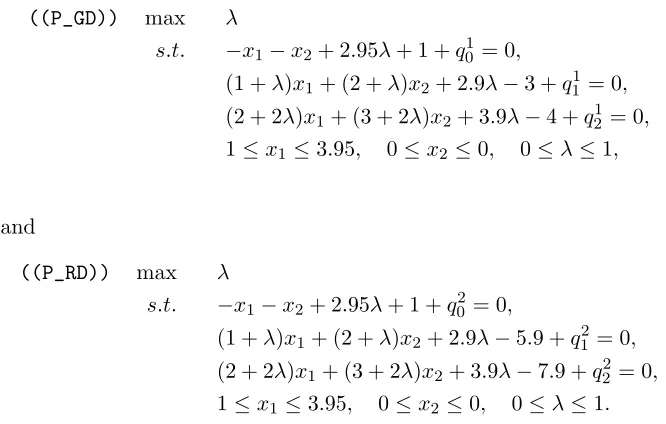
Now, bearing the solution of the latter subproblems in mind, we establish problems((P_GD))and ((P_RD))in the forms of
((P_GD)) max λ
s.t. −x1−x2+ 2.95λ+ 1 +q01= 0,
(1 +λ)x1+ (2 +λ)x2+ 2.9λ−3 +q11= 0,
(2 + 2λ)x1+ (3 + 2λ)x2+ 3.9λ−4 +q12 = 0,
1≤x1≤3.95, 0≤x2≤0, 0≤λ≤1,
and
((P_RD)) max λ
s.t. −x1−x2+ 2.95λ+ 1 +q20 = 0,
(1 +λ)x1+ (2 +λ)x2+ 2.9λ−5.9 +q21 = 0,
(2 + 2λ)x1+ (3 + 2λ)x2+ 3.9λ−7.9 +q22= 0,
1≤x1 ≤3.95, 0≤x2 ≤0, 0≤λ≤1.
We have solved((P_GD))and ((P_RD))firstly by using the fuzzy deci-sive set method and secondly by using the modified subgradient method.
• By the use of the fuzzy decisive set method, the solution of both problems ((P_GD)) and ((P_RD)) are obtained at the twenty first iterations, but with different optimal valuesλ20((P_GD))=
0.1574 andλ20((P_RD))= 0.4142.
• The results obtained by the use of the modified subgradient method are illustrated in Table 1 and Table 2.
Table 1. The results of using the modified subgradient method for solving((P_GD))
k uk0 uk1 uk2 ck xk1 xk2 λ H Hk kg(xk)k sk
1 0 0 0 0 1 0 1 0 -1 5.2462 0.0073
2 -0.0214 -0.0138 -0.0283 0.0743 1 0 1 0 -0.4100 5.2462 0.0029 3 -0.0302 -0.0195 -0.0400 0.1048 1 0 0.5102 0 -0.2345 1.8129 0.0142 4 -0.0517 -0.0193 -0.0544 0.1553 1.4635 0 0.1571 0 − 5.2×10⁻⁶ −
Table 2. The results of using the modified subgradient method for solving((P_RD))
k uk
0 u
k
1 u
k
2 c
k xk
1 x
k
2 λ H Hk kg(xk)k sk
1 0 0 0 0 1 0 1 0 -1 3.1149 0.0206
Once again remember that problems ((P_GD)) and ((P_RD)) have been generated according to the Gasimov and Yenilmez’s definition GD and the revised definition RDfor a fuzzy constraint, respectively.
Discussion. By comparing the results reported in Table 1 and Table 2, the following observations are evident: (i) The number of iterations for solving ((P_RD)), k = 3, is less than one for solving ((P_GD)),
k= 4. (ii) The satisfaction level of constraints in the problem((P_RD)) is more desirable than the counterpart in((P_GD)), becausekg(xk)k=
1.3×10⁻⁶ for((P_RD))is less than kg(xk)k= 5.2×10⁻⁶ for((P_GD)).
(iii) The maximum satisfaction degree of fuzzy decision set, that is, the optimum of((P_RD)),λ= 0.4142, has been more improved rather than the counterpart of((P_GD)),λ= 0.1571.
We note that all the above observations are in agreement with the results of the next experiment.
By the same manner as described in Example 1, we have examined the next example and consequently the results are summarized in Table 3 and Table 4.
Example 2. (Case 2.) Let
(pi) =
8 10
=⇒ (bi+pi) =
11 14
.
We have solved((P_GD))and ((P_RD))firstly by using the fuzzy deci-sive set method and secondly by using the modified subgradient method.
• By the use of the fuzzy decisive set method, the solution of prob-lems ((P_GD)) and ((P_RD)) are obtained at the twenty four first and at the sixteen first iterations, respectively, while optimal values areλ24((P_GD))= 0.0801 andλ16((P_RD))= 0.4143.
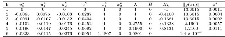
• The results obtained by the use of the modified subgradient method are illustrated in Table 3 and Table 4.
Table 3. The results of using the modified subgradient method for solving((P_GD))
k uk
0 uk1 uk2 ck xk1 x2k λ H Hk kg(xk)k sk
1 0 0 0 0 1 0 1 0 -1 13.6015 0.0011
Table 4. The results of using the modified subgradient method for solving((P_RD))
k uk0 uk1 uk2 ck xk1 xk2 λ H Hk kg(xk)k sk
1 0 0 0 0 1 0 1 0 -1 6.0828 0.0054
2 -0.0324 0.0054 0 0.0641 8.4852 0 0.4143 0 -0.4420 0.2×10⁻⁶ −
5. CONCLUSIONS
In this article we have suggested a revised formula for the member-ship function of fuzzy constraints involved in fuzzy linear programming problems with fuzzy technological coefficients and fuzzy right-hand side. Comparing the results obtained based on the Gasimov and Yenilmez’s formula and the revised formula indicates that the proposed formula has some advantages such as: the number of required iterations to get the desired solution is reduced; the maximum satisfaction degree of the fuzzy decision set reaches a more accurate optimum; and the sequence which evaluates how much constraints are violated, is controlled by a smaller upper bound.
References
[1] R.E. Bellman & L.A. Zadeh. ”Decision making in a fuzzy environment”. Man-agement Science. Volume 17, 141-164. (1970).
[2] R.N. Gasimov & A.M. Rubinov. ”On augmented Lagrangians for optimization problems with a single constraint”.J. Global Optimization. Volume 28, 153-173. (2004).
[3] R.N. Gasimov & K. Yenilmez. ”Sloving fuzzy linear programming problems with linear membership functions”.Turk. J. Math.,Volume 26, 375-396. (2002). [4] G.J. Klir & B. Yuan. ”Fuzzy sets and fuzzy logic-theory and applications”.
Prentice-Hall Inc., (1995).
[5] S. Mukherjee & Z. Chen & A. Gangopadhyay. ”A fuzzy programming approach for date reduction and privacy in distance-based mining”. Int. J. Information and computer Security, Volume 20, 27-47. (2008).
[6] N. Rafail & R.N. Gasimov. ”Augmented Lagrangian duality and nondifferen-tiable optimization methods in nonconvex programming”.J. Global Optimiza-tion, Volume 24, 187-203. (2002).
[7] N. Safaei & M.S. Mehrabad & R.T. Moghaddam & F. Sassani. ”A fuzzy pro-gramming approach for a cell formation problem with dynamic and uncertain conditions”. Fuzzy Sets and Systems, Volume 159, 215-236. (2008).
[8] M. Sakawa & H. Yana. ”Interactive decision making for multiobjective linear fractional programming problems with fuzzy parameters”.Cybernetics Systems, Volume 16, 377-397. (1985).
[9] T. Shaocheny. ”Interval number and fuzzy number linear programming”.Fuzzy Sets and Systems, Volume 66, 301-306. (1994).