Doctoral Thesis
School of Social Sciences
Doctoral School in Economics and Management
COMMODITY PRICE VOLATILITY:
Causes, Effects and Implications
a dissertation submitted to the doctoral school of economics and management in partial fulfilment of the requirements for the Doctoral degree (Ph.D.) in
Economics and Management
Harriet Kasidi Mugera
2
Supervisor:
Professor Christopher L. Gilbert Università degli Studi di Trento
Internal Evaluation Commission:
Professor. Giuseppe Folloni Università degli Studi di Trento Professor. Sara Savastano
Università degli Studi di Roma Tor Vergata
Examination Committee:
Professor Carlo Federico Perali University of Verona, Italy
Professor Luciano Fratocchi University of L’Aquila, Italy
i
TABLE OF CONTENTS
INTRODUCTION 1
CHAPTER I: VOLATILITY IN FOOD COMMODITY PRICES AND
THE COMOVEMENTS WITH CRUDE OIL PRICES 15
1. Have Commodities Become More Volatile? 18
2 The Co-movement of Crude Oil and Food Commodity Prices 23 3 The Generalised Autoregressive Conditional Heteroskedasticity Framework 33
4 Grains market volatilities 37
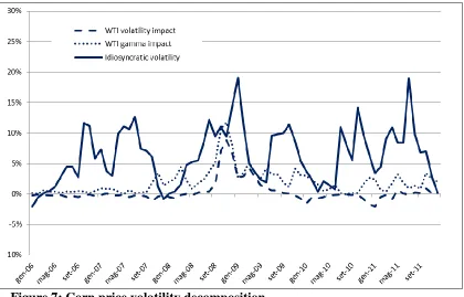
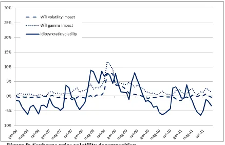
5 Volatility decomposition 46
6 Conclusions 52
CHAPTER II: STRUCTURAL CHANGE IN THE
RELATIONSHIP BETWEEN ENERGY AND FOOD PRICES 55
1. The relationship between food and energy commodities 56
2. U.S. biofuels policies 59
3. Structural break analysis 64
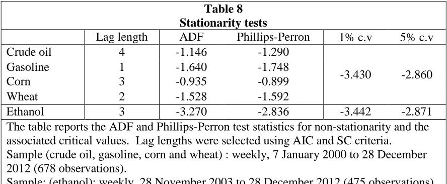
4. Data 75
5. Univariate test results 76
6. Multivariate test results 79
ii
CHAPTER III: POVERTY AND VULNERBILITY IN TANZANIA 99
1. Poverty and Vulnerability 102
2. Data and Methodology 121
3. Results 135
4. Conclusions 150
CONCLUSIONS 154
1
INTRODUCTION
Agricultural commodities experienced substantial increases in prices over the most
recent decade with major surges in both 2007-08 and again in 2010-11. The prices of
food commodities such as maize, rice and wheat increased dramatically from late 2006
through to mid-2008, reaching their highest levels in nearly thirty years. In the second
half of 2008, the price upswing decelerated and prices of commodities decreased
sharply in the midst of the financial and economic crisis. A similar price pattern
emerged in early 2009 when the food commodity price index slowly began to climb.
After June 2010, prices shot up, and by January 2011, the index of most commodities
exceeded the previous 2008 price peak. These price movements coincided with sharp
rises in energy prices, in particular crude oil. Sharp increases in agricultural prices were
not uncommon, but it is the short period between the recent two price surges that has
drawn concerns and raised questions. What were the causes of the increase in world
agricultural prices and what are the prospects for future price movements? Were the
trend driven by fundamental changes in global agricultural supply and demand
relationships that may bring about a different outcome? What are its implication on
global food security and sustainability?
Several authors have discussed the factors lying behind the sharp food price increases
over the period 2007-11 though no consensus has been reached on the cause of these
phenomena. Rapid economic growth in China and other Asian emerging economies,
decades of underinvestment in agriculture, low inventory levels, poor harvests,
2
among the factors cited as leading to high levels of commodity prices (Abbot et al,
2008, Cooke and Robles, 2009; Gilbert, 2010; Wright, 2011). In addition to the above
mentioned factors, the diversion of food crops as bio-fuels stands out as an important
and new factor that many have seen as accountable for the food price spikes (Mitchell,
2008).
The price spikes were also associated with increased price volatility in commodity
prices. Increasing volatility has been a concern for most agricultural producers and for
other agents along the food chain as it renders planning very difficult for all market
participants. Price volatility can have a long run impact on the incomes of many
producers and the trading positions of countries and can make planning on production
more difficult. As argued by Aizenman and Pinto (2005), higher volatility results in an
overall welfare loss, though some may benefit from higher volatility. Sudden changes
and long run trend movements in agricultural commodity prices present serious
challenges to market participants and especially to commodity dependent and net food
importing developing countries (FAO 2010). At the national level, food-importing
countries face balance-of-payment pressure as the cost of food imports rise. When
transmitted to domestic markets, high world prices erode the purchasing power of urban
households and other net food buyers (Minot, 2009). Moreover, adequate mechanisms
to reduce or manage risk to produces may not exist in some markets and countries or are
not easily accessible in others.
Primary commodity prices are variable because short term production and consumption
elasticities are low. On the supply side, production responsiveness is low in agriculture
because input decisions are made before new crop prices are known. These decisions in
3
consumption elasticities, and particularly short-term demand are low because actual
commodity price may not be a large component of the overall value of the final product.
Low elasticities thus imply that small shocks in production could have substantial price
impact.
In agriculture, volatility in food prices is of particular importance as can be noted from
different perspectives. Firstly, most of the poor households in developing countries
spend large proportions of their incomes on food. Secondly, most farm households in
developing countries are small-scale farmers who sell their produce onto the market but
also happen to be net buyers. Thirdly and lastly, most small-scale farm households fully
rely on the sale of food commodities in order to cover their basic needs and
expenditures like health and education expenses. Food price volatility thus feeds
directly into the dynamics of poverty. This is so since high food prices can play a major
role in moving many vulnerable non-poor households into poverty and low food prices
can move non-poor farm households into poverty. Since these households devote a large
proportion of their budgets to food price shocks can easily pre-empt their income
moving them from sustainability into poverty (Anderson and Roumaset, 1996).
The sudden and unexpected rise in world food prices in recent decade has drawn the
attention of policy makers to agriculture and this has led to the debate about the future
reliability of world markets as a source for food. The fear of further spells of volatility
in food prices has prompted efforts in designing and proposing price stabilizing
mechanisms both at international and national levels. This fear has been driven by the
recognition that a new set of forces may be driving drive food prices and their volatility
trend. These forces emerge from linkages between the agricultural and the energy
4
macroeconomy, which together, render agricultural markets much more exposed to
shocks.
Previous research has shown that in the recent decade there has been an increase in
volatility grains, vegetable oils and meats. These are commodities which are likely to be
affected by the growth of biofuel production. On this view, heightened food price
volatility arises due to the importation of oil price volatility. Despite this, crude oil price
volatility has not been particularly high over the period considered. This suggests that
the relationship between crude oil and grains prices may have changed over the most
recent decade resulting in greater transmission of oil price volatility into grains prices.
Consistent with this view, grains and crude oil returns have in the recent years been
co-moving as shown by the increased correlations between the two groups. These increased
correlations may be accounted for either in terms of an increase in the pass-through
from the crude oil market to the grains markets or by an increased prevalence of
common shocks across the two sets of markets (Tyner, 2010; Serra et al., 2011c; Gilbert
and Mugera, 2013)
Increased biofuel production and consumption over the recent decade may have created
a new demand side link between energy markets and food commodities by making the
demand for grains and vegetable oils sensitive to the price of crude oil. In the United
States biofuel production began to rise rapidly in 2003 while in the European Union it
accelerated from 2005 (USDA, 2008). Ethanol production (mainly in the United States
and Brazil) tripled from 4.9 billion gallons to almost 15.9 billion gallons between 2001
and 2007. In the U.S., corn production used for ethanol production increased from 12.4
5
2011). Over the same period, biodiesel production, mainly in the European Union and
deriving from vegetable oils, rose almost ten-fold, to about 2.4 billion gallons.
A number of authors have documents the increased co-movement and correlation
between crude oil prices and food commodity prices over the most recent decade
(Tyner, 2010; Serra et al., 2011c; Gilbert and Mugera, 2013). This increase in
co-movement appears to have commenced at around the same time as biofuels production
took off.
Observers have claimed that the demand for food commodities – in particular, corn,
sugar, and vegetable oils – for use as biofuels feedstocks has increased the demand and
prices of food commodities (Mitchell, 2008). Agricultural economists for the World
Bank and United States Department of Agriculture estimated the share of biofuels’
contribution to explaining high grain prices since mid-2007 at between 60 to 75 percent
respectively (Mitchell, 2008). Academic analysts on the other hand, placed the share at
between 25 and 35 percent (Rosegrant, 2008)1. Other commentators were more
sceptical about the price impact of biofuels production – see Gilbert and Morgan
(2010). They emphasize that biofuels demand may have increased the magnitude of the
demand side shocks (that were imported from the energy markets) and reduced the
demand elasticity due to restrictive and inflexible mandates.
The hikes in fuel and energy prices are structural as they reflect a long-term imbalance
between rising incremental oil demand and relatively stable production and supply
(ADB, 2008). Energy prices may affect food commodity prices in two ways. Firstly, an
1 The IMF estimated that during the commodity spike, the increased demand for biofuels accounted for 70
6
increase in oil prices exerts more pressure on the production cost through fuel used in
tractors and transportation as well as pesticides and fertilizers used in agriculture. This
will in turn lead to an upward shift of the supply curve. This pass-through process will
partly be through the costs of nitrogen-based fertilizers and partly through transport
costs. However, agriculture is not highly energy intensive. Baffes (2007) estimated the
pass-through of oil prices into agricultural commodity prices as 17% and this has not
changed much over time (Gilbert 2010). Mitchell (2008) estimated 15 – 20% in
agricultural production costs in the US was due to the combined effects of higher
energy and transport costs.
Secondly, high crude oil prices stimulate biofuel production and increases the demand
for agricultural commodities, in particular corn and oil seed rape. This increase results
in a rightward shift in the demand curve due to the new demand for food commodities
as biofuel feedstocks (Gilbert, 2010). The result is that shocks from the energy demand
are transmitted into the food commodities. This then increases the variability of food
prices as well as the correlation to energy prices. This increased correlation is predicted
by models which emphasize the demand for corn as a biofuel feedstock. In these
models, provided the corn price in the absence of biofuels demand allows profitable
conversion to biofuels, a rise in the price of crude oil pulls up the corn price – see
Schmidhuber (2006). Substitution of land across crops generalizes the corn price
increase to other commodities such as wheat and soybeans. Soybeans are most directly
affected by the demand for corn-based ethanol as corn and soybeans tend to compete for
land area and can be used in rotation. Thus an increase in the demand for corn could
7
The expansion in biofuels production has been driven by a number of economic and
environmental factors. High crude oil prices and keenness to promote non-petroleum
energy sources to reduce dependence on oil imports have been important policy drivers
in the United States, Brazil, and the European Union. Environmental concerns over
greenhouse gas emissions and the urge to slow down global warming due to fossil fuel
emissions have also contributed to this expansion. Debate remains on whether the
increase in biofuels production was primarily market or policy-driven. Some authors
believe that the boom was mainly driven by the increase in crude oil prices. Others
sustain that the boom resulted from government policies, such as mandates and tax
credits in the U.S. aimed at increasing energy self-sufficiency and, in Europe,
environmental pressures to reduce emissions (DeGorter and Just, 2009; Abbot, 2013;
Peri and Baldi, 2013).
In particular in the United States, July 2005 marked the beginning of what Abbot (2013)
termed as the “ethanol gold rush which coincided with policy interventions such as the
2005 Renewables Fuels Standards was enacted (U.S. Congress, 2005). In 2007 then
followed the Energy Policy Act which significantly increased the mandated RFS
minimum levels of ethanol production (U.S. Congress, 2007). Tyner (2010) confirms
that the correlation between energy and agricultural markets has been strong since the
2006 start of the ethanol boom. He highlights the summer of 2008 as the period where
these two markets were closely linked. As the crude oil price increased so did the price
of corn and other agricultural commodities.
Increasing globalisation and market liberalisation have fostered linkages between
markets and have thus influenced volatility in individual markets. To some extent,
8
determining major price shocks but whether this will turn out to be the pattern for future
volatility developments still remains unclear. In particular, we have observed strong
linkages between international and domestic markets in countries that trade on
international markets. Most developing countries consume grains such as corn and
wheat (mainly in East Africa and rice (in most of West Africa) as staples. Most of these
countries are not self-sufficient and thus depend heavily on either direct (through
international markets) or indirect imports (through regional markets). Shocks in
international markets are therefore transmitted to domestic markets (Rapsomanikis and
Mugera, 2011). Recent food spikes in international markets mainly affected grains such
as corn, wheat, rice and soybeans. Increased international food commodity prices were
in large measure transmitted back to domestic markets in developing countries where
poor households, particularly those in urban areas, spend a large proportion of their
incomes on food (World Bank, 2008) thus threatening food security and poverty (FAO,
2008).
Governments as well as policy makers are becoming more and more aware that policies
that help households manage risks and cope with shocks should form an integral part of
poverty eradicating strategies (Holzmann and Jorgensen, 2001). The renewed focus by
policy makers to address risk and vulnerability in formulating policies to reduce poverty
has motivated a series of studies aimed at measuring and assessing household
vulnerability empirically.
While it is increasingly recognized that household vulnerability mitigating interventions
must be an integral part of any poverty reduction strategy (World Bank, 2001), the
quantitative links between risks and poverty have not been fully documented. Risk and
9
Risks contribute to poverty dynamics in a number of ways. Firstly, risks may blunt the
adoption of technologies and strategies of specialization necessary for agricultural
efficiency (Carter, 1997). Risks may drive farmers to apply less productive technologies
in exchange for greater stability (Morduch, 2002, Larson and Plessman, 2002).
Secondly, risks may function as a mechanism for economic differentiation within a
population, deepening poverty and food insecurity of some individuals even as
aggregate food availability improves (Carter, 1997).In the absence of risk management
instruments, risk events may plunge highly vulnerable households into poverty
(Holzmann and Jorgensen, 2000). From a policy perspective, risks are detrimental to the
welfare of (poor) households and that ensuring security is an essential ingredient of any
poverty alleviation strategy (World Bank, 2001). A household facing a risky situation is
subject to future welfare loss. The likelihood of experiencing future loss of welfare,
generally weighted by the magnitude of expected welfare loss, is called vulnerability
(Sarris and Panayiotis, 2006).
Poverty and vulnerability are basic aspects of well-being. Exposure to risk and
uncertainty about future events and its adverse effects to wellbeing is one of the central
views of the basic economic theory of human behavior, embodied in the assumption
that individuals and households are risk averse. Most poverty and vulnerability
measures are unidimensional, focusing on a single measure of wellbeing such as income
or consumption expenditure to identify who is poor or vulnerable. There is need to
develop a multi-dimensional measure that incorporates different aspects of poverty
especially for poor and developing countries. Ligon (2008) empirically shows that the
main consequence of increased food prices is that poor consumers, that devote a larger
10
expenditures such as investments in health, education, as well as other non-food items.
The negative impact of high food prices is not highly visible in a reduction of food
consumption but is likely to be visible in other dimensions such as decreases in
schooling rates, health expenditures, and other similar investments, as the need to
purchase food at higher prices overwhelms the need to spend on other goods. This result
not only questions the use of food consumption as a proxy to poverty and vulnerability
as it also prompt the need to incorporate other issues of household’s well-being that
may be affected when households are hit by shocks such as high food prices.
Policy makers are mainly interested in applying appropriate forward-looking
anti-poverty interventions (i.e., interventions that aim to go beyond the alleviation of current
poverty to prevent or reduce future poverty), the critical need thus to go beyond a
classification of who is currently poor and who is not, to an assessment of how
households’ are vulnerability to poverty. Creating awareness of the potential of such
irreversible outcomes may drive individuals and households to engage in risk mitigating
strategies to reduce the probability of such events occurring. Moreover, focusing on
vulnerability to poverty serves to distinguish ex-ante poverty prevention interventions
and ex-post poverty alleviation interventions. Policies directed at reducing
vulnerability–both at the micro and macro level– will be instrumental in reducing
11
The first chapter of this thesis examines food and energy commodity price volatility
over the past decade. The objective of this chapter is to analyse the evolution of this
relationship considering the role played by biofuels. It aims at verifying whether the
increased grains-crude correlations has led to greater grains volatility as shocks from the
crude oil markets are transmitted into the grains market. If this is the case, one would
expect there to be a pass-through mechanism of crude oil shocks into the grains
markets.
It focuses on two main issues. Firstly, it establishes whether food and energy
commodity markets have become more volatile in recent times. Secondly, it analyses
the nature of relationship between food and crude oil prices. In particular, it
investigates whether the volatility in food commodities is now driven by the
transmission of shocks from the crude oil market as a result of increased biofuel
production and consumption. A short and a long term historical volatility measure are
calculated for different commodities in order to evaluate whether commodity markets
have become more volatile in recent times. Multivariate General Autoregressive
Heteroskedasticity (MGARCH) models are implemented to establish the nature of the
relationship between food and energy prices. Using estimates from the Dynamic
Conditional Correlation (DCC) Multivariate GARCH models specification, it
decomposes volatility of food commodities into its main components. Conditional
correlations are calculated from MGARCH models estimated on daily data over the
twelve year sample 2000-2011. Increased commodity comovement implies a rise in
inter-commodity correlations. An advantage of the DCC framework is that it allows the
investigator to focus specifically on changes in pass-through from the crude oil market
12
The second chapter of this thesis focuses on the structural changes in food and energy
prices and price relationships given the role of biofuels and biofuel policies in the
United States. Increases in energy prices, the boom in biofuel production and
government policy interventions have led to questions in relation to the stability in the
long run relationships between food and energy commodity prices. This chapter
investigates the assertion that the advent of biofuels has altered the nature of the
relationship between energy and agricultural markets. The main hypothesis of this
second chapter is that recent market and policy events may have induced changes in the
relationship between food and energy markets.
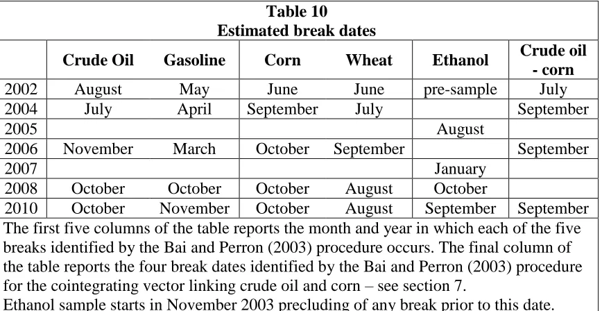
Using the Bai and Perron structural break methodology this chapter analyses price
relationships between grains and energy prices over the period since 2000 and relates
the structural breaks to changes in U.S. biofuel policy. It thus tests whether there have
been any structural changes in relationships between energy and commodity prices and
if so, whether any such breaks may be modelled as shifts in the mean of the food price
processes. It further tests for the presence of multiple structural breaks in the single
price series of crude oil, gasoline, ethanol corn, and wheat without pre-specifying the
dates of any such breaks. The main focus of this chapter is the United States. This
choice is driven by several factors. Firstly, the United States is one of the largest
producers and exporters of grains and oilseeds. Secondly, the United States is the
world’s largest producer and consumer of biofuels. Thirdly, in the recent decade, the
United States has experienced a large number of policy and regulatory changes that may
13
The third chapter quantitatively assesses households’ welfare dynamics in the recent
years. Given the recent international shocks and market related shocks, the objective of
this chapter is to quantitatively assess poverty and vulnerability dynamics in Tanzania.
This chapter generates a unidimensional and a multidimensional poverty indicator. The
Multi-dimensional Poverty Indicator (MPI) is generated implementing the Alkire and
Foster (2011) multidimensional methodology. This measure proposes a dual cut-off at
the identification step of poverty measurement and it provides an aggregate poverty
measure that reflects the prevalence of poverty and the joint distribution of deprivations.
Based on the above poverty indicators this chapter runs a series of logit models for the
2008-09 and 2010-11 survey conditioned upon covariates of 2008-09 and 2010-11
respectively. These include household characteristics including asset ownership,
geographical attributes such as location in rural or urban settings and shocks. The
models are run using the MPI poverty measure and our baseline measure which is
consumption expenditure (income poverty indicator). Using both a unidimensional a
multidimensional poverty measure, we analyse both poverty and vulnerability in
Tanzanian households.
Tanzania is selected as the country of analysis because maize is the staple food in all
households. Maize is one of the food commodities most severely affected by the recent
food spikes. Tanzania has also been recently both economically and politically stable
and is thus conducive for conducting a survey analysis. Tanzania is a relatively large
country and also trades on the international markets. Household quantitative and
qualitative information have also been well documented for the relative period of
14
survey panel datasets that have been collected and compiled by the Living Standards
Measurement Study (LSMS-ISA, World Bank).
To understand poverty, it is essential to examine the economic and social contexts of the
households which include the characteristics of local institutions, markets, and
communities. Poverty differences cut across gender, ethnicity, age, rural versus urban
location, and income source. Rural poverty accounts for nearly 63 percent of poverty
worldwide, and is between 65 and 90 percent in sub-Saharan Africa (IMF, 2001). This
15
CHAPTER 1:
VOLATILITY IN FOOD COMMODITY PRICES AND THE
CO-MOVEMENT WITH CRUDE OIL PRICES
In 2008, the world experienced a dramatic surge in the prices of commodities. The
prices of food commodities, in particular maize, rice and wheat increased dramatically
from late 2006 through to mid-2008, reaching their highest levels in nearly thirty years.
Prices stabilized in the summer of 2008 and then decreased sharply in the midst of the
financial and economic crisis. A similar price pattern emerged in early 2009 when the
food commodity price index slowly began to climb. After June 2010, prices shot up, and
by January 2011, the index of most commodities exceeded the previous 2008 price
peak. Sharp increases in agricultural prices are not uncommon, but it is rare for two
price spikes to occur within 3 years as they normally occur with 6-8 year intervals. The
short period between the recent two price surges has therefore drawn concerns and
raised questions. What are the causes of the increase in world agricultural prices and
what are the prospects for future price movements? Will the current period of high
prices end with a sharp reversal as in previous price spikes, or have there been
fundamental changes in global agricultural supply and demand relationships that may
16
A number of authors have discussed the factors lying behind the spikes though no
agreement has been reached on the cause of these phenomena. Rapid economic growth
in China and other Asian emerging economies, decades of underinvestment in
agriculture, low inventory levels, poor harvests, depreciation of the U.S. dollar, and
speculative influences are some of the factors considered and cited as leading to high
levels of commodity prices. In addition, the diversion of food crops as bio-fuels stands
out as an important and new factor that many have seen as accountable for the food
price spikes.
The recent price spikes were also accompanied by volatile commodity prices. There is
evidence of increased price volatility from mid-2000 for most food commodities in
particular those of grain prices. Price volatility in commodities has been considerable,
making planning very difficult for all market participants. Sudden changes and long run
trend movements in agricultural commodity prices present serious challenges to market
participants and especially to commodity dependent and net food importing developing
countries. At the national level, food-importing countries face balance-of-payment
pressure as the cost of food imports rise. When transmitted to domestic markets, high
world prices erode the purchasing power of urban households and other net food buyers.
Poor urban households are particularly affected because they spend a large share of their
income on food.
A majority of analyses examining biofuels impacts on energy and food commodity
markets have focused the attention on price-level links while price volatility has
received much less attention. An increased correlation between food and energy prices
is likely to yield stronger volatility spillovers between prices in these two markets. The
17
which can usefully complement the larger body of research which looks at price level
impacts.
The aim of this chapter is to analyse the nature and cause of food commodity price
volatility. It has two main objectives. Firstly, it establishes whether commodity markets
have become more volatile in recent times. Secondly, it analyses the nature of
relationship between commodity and crude oil prices. In particular, it aims at studying
the evolution of this relationship considering the role played by biofuels. A short and a
long term historical volatility measure are calculated for different commodities in order
to evaluate whether commodity markets have become more volatile in recent times. It
investigates whether the volatility in food commodities is now driven by the
transmission of shocks from the crude oil market as a result of increased biofuel
production and consumption. This chapter employs Multivariate General
Autoregressive Heteroskedasticity (MGARCH). Conditional correlations are calculated
from MGARCH models estimated on daily data over the twelve year sample
2000-201Using estimates from the Dynamic Conditional Correlation (DCC) Multivariate
GARCH models specification, it decompose volatility of food commodities into its
main components. An advantage of the DCC framework is that it allows one to focus
specifically on changes in pass-through from the crude oil market to the grains markets.
This chapter focuses on grains food commodities since these are overall the most
important food crops. Grains are the major staple food across the globe and also are
an input into the production of meat products. Moreover, grains were the main
commodities that have been affected in the recent food spikes and are thus are crucial
18 It examines the prices of:
Maize (corn): The analysis of corn price volatility is for three reasons. First,
maize (white) is a staple food in eastern and southern Africa. Second, it forms
the main ingredient in animal feed in the United States. Third, it is the main
biofuel feed stock in the United States;
Wheat: It is the most important grain in temperate regions; in recent times it
has been used as a substitute to maize in animal feed;
Soybeans: It is important both as an animal feedstock and, when crushed, as a
vegetable oil. It also competes for land with corn in the United States.
1. HAVE COMMODTIES BECOME MORE VOLATILE? 1.1Volatility in food commodity prices
An increase in food commodity price volatility can be due to one or more of the
following four factors:
An increase in the variance of demand shocks; the diversion of food crops into
biofuel production could lead to increased demand variability. Increased
demand for food commodities, in particular corn, in the recent decade sugar
and vegetable oils, as biofuel feedstocks has increased the correlation between
agricultural prices and the oil price. This allows transmission of oil price
volatility to agricultural prices, in effect increasing the variance of demand
shocks;
An increase in the variance of supply shocks; Poor harvests such as those
19
2007 harvest have been mentioned as possible causes of the recent food price
spikes. However, these poor harvests were offset by good harvests elsewhere
in the world, notably Argentina, Kazakhstan and Russia, and 2008 harvests
were good;
A decline in the elasticity of demand; elasticity in demand depends on the
response of consumers to price changes and this in turn depends on the price
transmission i.e. the extent to which prices on world markets are passed
through to local prices. Government interventions such as subsidies in
response to higher food prices may diminish price responsiveness on the part
of consumers thus rendering markets and prices highly inelastic. US
government policy interventions through tax credits, mandates and subsidies
have been identified as some policy interventions that affected the
responsiveness of corn and biofuel markets to changes in crude oil and
gasoline prices;
A decline in the elasticity of supply: Grain inventories have fallen over time
since the millennium. Increased demand for corn and other feeedstocks for
biofuel production have in turn reduced the responsiveness of supply to the
demand shocks thus increasing volatility in these commodities.
1.2 Historical Volatility
Many commentators have maintained that commodity markets have generally become
more volatile over the recent decade compared to the past. In this section of the chapter
we look at the volatility of agricultural food commodity and crude oil prices both over a
20
i.e., the standard deviation of monthly price returns, over each calendar year. Monthly
returns are converted to an annual rate by multiplying by 2. We conduct both a long
term and short term volatility analysis. In the long-term volatility analysis we compare
the volatility measures of two-decade samples i.e., 1970-1989 with 1990-2011. In the
short term analysis we compare volatilities between two- five year sub-samples, i.e.,
2000-2006 and 2007-2011.The main data sources are the International Financial
Statistics of the IMF and the Chicago Board of Trade (CBOT).
Historical Volatility in Commodity Markets
Gilbert and Morgan (2010) compared volatilities of food commodity prices over the two
decades 1990-2009 with those over the immediately prior two decades 1970-1989. For
the majority of the commodities they considered, volatility was lower in the later period,
and in many cases this decline was statistically significant. We update the analysis by
comparing 1970-89 with 1990-2011 and include crude oil to this comparison. The
results are similar to those reported by Gilbert and Morgan (2010).
Figure 1 shows that even if volatility has risen recently, it remains substantially lower
than in the 1970s. Importantly, crude oil prices show a significantly lower volatility in
the later period relative to the earlier. Crude oil prices appeared to be more volatile in
the 1970-1989 sub-period as compared to the 1990-2010 sub-period. There is a 4
percentage point statistically significant difference in the volatility measure between the
two sub-samples.
2 It is convenient to use this standard conversion factor as it is in line with the efficient market theory of
21
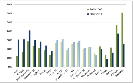
Turning to the shorter comparison of 2007-11 against 2000-06, there is clear evidence
that volatility for some commodities has increased – see Figure 2. Specifically,
volatility shows a significant increase for seven out of 19 food commodities analysed.
There are significant volatility increases for all four grains considered (maize, rice,
sorghum and wheat), and also for sunflower oil and beef. Other agricultural
commodities either show a volatility decrease or a statistically insignificant increase.
For purposes of comparison, crude oil prices show a small and statistically insignificant
rise in volatility over the same period.3
One can therefore conclude that although there has not been any general increase in
agricultural price volatility, there has been an increase in the volatility of grains prices
and that this increase extends to some vegetable oils and meat prices. Despite this, food
price volatility remains lower than in the 1970’s. The concentration of volatility
increases on grains, sunflower oil and beef is consistent with biofuels, having played a
major role. Notably, however, there does not appear to be a significant increase over
this comparison period in crude oil volatility4.
3 This comparison is based on an average of WTI and Brent prices on the basis that the WTI price was the
more representative of world oil price is the first part of the period but, because of limitations in storage capacity at the Cushing (OK) hub, Brent became the more representative price in the final years of the sample.
4 Similar results are obtained for the some of the metals. In the long-run comparison, aluminium and
22
Figure 1: Volatilities 1970-89 and 1990-2011
23
2. THE CO-MOVEMENT OF CRUDE OIL AND FOOD COMMODITY PRICES
2.1 Crude Oil and Commodity Markets
Global biofuel production has increased rapidly over the last 20 years. In the US this
began to rise rapidly in 2003 while in the EU it accelerated in 2005 (USDA, 2008).
According to FAO (2008), demand for cereals for industrial use, including biofuels,
rose by 25 percent from 2000 to 2008 against a 5 percent increase in global food
consumption. Moreover, increased biofuel production contributed to a 97 percent
increase of the price of vegetable oils in the first three months of 2008 (FAO, 2008).
Crude oil prices can affect the prices of food commodities in two distinct ways. First,
crude oil enters the aggregate production function of most primary commodities through
the use of various energy-intensive inputs such as fertilizers, heating, pesticides and
transportation. However, agriculture is not highly energy-intensive so this impact is
unlikely to be large and there is no reason to suppose that it has increased markedly in
recent years.
Secondly, some commodities can be used to produce substitutes for crude oil. This is
true in particular for maize and sugarcane in ethanol production and oil seed rape and
other vegetable oils for biodiesel production. The attractiveness to produce ethanol and
biodiesel, and to invest in refining capacity to produce these products, depends directly
on the price of crude oil. One should thus expect to find a relationship between food
commodity prices and crude oil prices. Although the impact of higher crude prices on
the demand and supply of grains and oilseeds takes time, efficient futures markets
24
2.2 Price Co-movement: Correlations
A number of authors have emphasized the increased co-movement of food prices (and
indeed on commodity prices generally) with crude oil prices, stock market returns and
exchange rate changes over the recent past. There is little dispute in relation to the facts.
Büyükşahin, Haigh and Robe (2010) document that the correlation between equity and
commodity returns increased sharply in the latter part of 2008 following the Lehman
collapse. UNCTAD (2011) reports that the rolling correlation between crude oil returns
and returns and on the S&P 500 equity index has grown steadily since 2004. Tang and
Xiong (2012) find similar rises in the rolling correlations between crude oil returns and
both agricultural and non-agricultural commodity futures prices. Bicchetti and Maystre
(2012) use high frequency data to document a jump in the moving correlation in the
returns on various commodity futures (including CBT corn, soybeans and wheat, CME
live cattle and ICE sugar) and S&P 500 futures returns.
Gilbert and Mugera (2012) show that the conditional correlations, generated from a
multivariate Dynamic Conditional Correlation (DCC) GARCH model (see Engle,
2002), between daily returns on WTI crude oil and respectively CBOT corn, soybeans
and wheat rose sharply from around 2006.
We estimate monthly logs averages of agricultural food commodities and Brent (ICE)
crude oil prices. We then estimate and statistically test the correlations between the two
sets of prices. The correlations are estimated for two sub-periods 2000-06 and 2007-11.
25
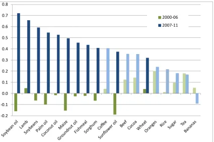
statistically significant. These estimates are charted and represented in Figure 3. Dark
colours indicate statistically significant increases in correlation (at the 5% significance
level).
With the single exception of bananas, price changes are all positively correlated with
changes in the price of crude oil in the 2007-11 sub-period while in the earlier period
they are small and do not exhibit any consistent sign. The correlation between crude oil
and the commodities increases from 2000-06 to 2007-11 with the exception of the crude
oil-bananas correlation. 11 out of 19 of the increased correlations are statistically
significant. This is particularly the case for all the grains except rice, all the oil seeds
and additionally for lamb. This is the same broad group of food commodities for which
the volatility increases were seen as significant.
-0.2 -0.1 0.0 0.1 0.2 0.3 0.4 0.5 0.6 0.7 0.8
2000-06 2007-11
26
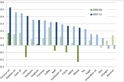
Figure 4 repeats the same exercise substituting S&P industrial monthly returns for crude
oil price changes. The same pattern of increased correlations can be observed but in this
case, the magnitude of the 2007-11 correlations are generally lower (except for coconut
oil) and very few of the increased correlations observed and tested are statistically
significant ( only 6 out of 11 are statistically significant).
-0.3 -0.2 -0.1 0.0 0.1 0.2 0.3 0.4 0.5 0.6
2000-06 2007-11
Figure 4: Correlations, Changes in Food Prices and S&P Returns, 2000-06 and 2007-11
The correlations reported in Figures 3 and 4 demonstrate that the increase in
co-movement between agricultural food commodities has been more dramatic with crude
oil prices than that with share prices. Since changes in crude oil prices are themselves
correlated with equity returns, it seems possible that co-movement of food commodity
27
and Maystre (2012) may be largely accounted for as an indirect impact of changes in
crude prices.
We therefore estimate and statistically test the partial correlations first of food
commodities and equity, holding crude oil prices constant and then food commodities
with crude oil, holding equity returns constant.. Table 1, which reports the partial
correlations of food commodity prices and respectively crude oil prices and equity
returns, demonstrates that this is indeed correct. The partial correlations of food
commodity prices and the equity returns, holding crude oil prices constant, showed only
a modest increase between 2000-06 and 2007-11 (Table 1, columns 3 and 4) while that
between food commodity and crude oil prices, holding share prices constant, rose
sharply (Table 1, columns 1 and 2).
It is therefore the increased comovement of food commodity crude oil prices which
requires explanation, as emphasized by UNCTAD (2011), Tang and Xiong (2012) and
Gilbert and Mugera (2012) provide two rival explanations. Tang and Xiong (2012) see
this as a financialization effect. According to their view, the increased correlation arises
as index investors buy or sell “on block” the entire range of commodity futures included
in the two major commodity indices of which crude oil is the single most important by
index weight. They claim that the comovement is greater for commodities included in
indices than for those less liquidly contracts outside the indices. Figure 5 fails to bear
out this contention with respect to the comovement of food commodity and crude oil
28
The alternative view, stressed by Gilbert and Mugera (2012), is that the comovement
arises instead from the biofuels link whereby the profitability of diverting grains
(essentially corn) into ethanol production and vegetable oils (largely oil seed rape and
29
Table 1 Partial Correlations
Brent crude S&P Industrials
2000-06 2007-11 2000-06 2007-11
Cocoa 0.1277 0.2615 -0.0762 0.2615
Coffee 0.0883 0.3007 0.2604 0.1428
Tea 0.1833 0.0686 0.1058 0.1673
Sugar 0.1105 0.1204 0.0889 0.0794
Oranges 0.2163 0.3013 0.1068 -0.1934
Bananas 0.0768 -0.0755 0.0500 0.0000
Beef 0.1131 0.2387 0.0566 0.1808
Lamb 0.0200 0.5739 -0.1616 0.1304
Wheat 0.0000 0.2360 -0.2313 0.1058
Rice 0.0624 0.1944 0.0100 -0.0100
Maize -0.1513 0.4343 0.0000 0.0283
Sorghum -0.0624 0.2879 0.0100 0.1903
Soybeans 0.0500 0.5138 0.0742 0.0900
Coconut oil 0.0141 0.3604 0.1726 0.3633
Soybean oil -0.1378 0.6392 0.1288 0.1764 Groundnut oil -0.0283 0.4441 -0.0100 -0.0964
Palm oil -0.0707 0.4199 0.1606 0.2410
Sunflower oil -0.1720 0.2782 0.0933 0.1304
Fishmeal 0.0000 0.3245 0.0943 0.1694
Average 0.0232 0.3117 0.0491 0.1135
Columns 1 and 2 give the partial correlations of the change in the row price holding the
Brent crude price constant. Columns 1 and 2 give the partial correlations of the change in
the row price holding the S&P Industrials index constant. Bold face indicates statistical
30
2.3 Effects of Biofuels
Biofuels have two main distinguishable effects. The first effect is that it raises the price
levels due to diversion of supplies from food and feed consumption. This happens
directly via competition between food and feed users and biofuel users for the same
grain, but also indirectly, through the substitution of one grain, such as maize diverted
to biofuel feedstock from use as food or feed rations, leading to substitution of a food
grain, such as wheat, into animal feed. Soybeans are most directly affected by the
demand for corn-based ethanol as corn and soybeans tend to compete for land area and
can be used in rotation5 .
The U.S. expanded maize area by 23 percent in 2007 in response to high maize prices
and rapid demand growth for maize for ethanol production. This expansion resulted in a
16 percent decline in soybean area which reduced soybean production and contributed
to a 75 percent rise in soybean prices between April 2007 and April 2008. The
expansion of biodiesel production in the EU diverted land from wheat and negatively
affected wheat production and stock levels. This was in response to the increased
demand and rising prices for oilseeds, land cultivated for oilseeds - particularly rapeseed
- increased. Oilseeds and wheat are grown under similar climatic conditions and in
similar areas and most of the expansion of rapeseed and sunflower displaced wheat or
was on land that could have been used for wheat cultivation (Mitchell, 2008).
Grains prices also affect the price of meat and dairy products because grain is used as
feed. Livestock feeding is the largest single use of corn and cattle, hogs, and poultry all
use corn feed, thus the expansion in the ethanol industry does affect livestock
5 In 2007-2008, the price of corn rose substantially reflecting the increase in demand, the cropping pattern
31
production. Prices will adjust quickly for some such as chicken, milk and eggs, but take
more time for others such as beef and pork. The price adjustment period reflects the
length of time farmers need to adjust their stock (supply) in response to the higher feed
prices (Gilbert 2010).
The second effect of biofuels is it may increase the volatility of food prices. Gilbert and
Morgan (2010) note that the volatility of any commodity price depends on the variances
of shocks to production and consumption in conjunction with the elasticity of supply
and demand. Within this framework, the biofuels link may be seen as introducing an
additional source of demand variability – see Wright (2011) who emphasizes the
transmission of energy market shocks into food commodity markets – and, if biofuel
mandates are inflexible, as decreasing demand elasticities. The main focus of the current
chapter is on these volatility links.
2.4 Linkages between Commodity and Crude Oil Markets
The direct production function that links crude oil prices to food commodity prices is
well-documented. Using different methodologies, Baffes (2007), Mitchell (2008) and
Gilbert (2010) agree in seeing an energy price pass-through to grains prices of between
15 and 20 per cent. It is unlikely that this has changed over recent years. The indirect
links, via the use of food commodities as biofuel feedstocks, are more difficult to
quantify, in part because of the shortness of the relevant biofuels time series. Moreover,
few of the formal models have been able to capture the cross-commodity supply and
demand linkages between corn – the primary grain used to make ethanol – and other
32
Gilbert (2010) used Granger-causality (GC) tests to examine the link between crude oil
prices and both the IMF’s agricultural food price index and a grains sub-index. In both
cases, his results showed a negative impact Granger-causal in the two decades up to
1989 and a positive Granger-causal impact in the two more recent decades. The
pre-1989 results may reflect the fact that, over that period, the developed economies lacked
a clear monetary anchor and hence a rise in oil prices would likely be met by a tough
anti-inflationary monetary tightening. The production function pass-through-impact of
higher oil prices only becomes apparent once the credibility of inflation targeting had
been established.
Tyner (2010) confirms that since the ethanol boom took off in 2006, the correlation
between energy and agricultural markets has been strong. He highlights the summer of
2008 as the period where these two markets were closely linked. As crude oil price
increased so did the price of corn and other agricultural commodities. And when crude
oil prices started to decline after the summer of 2008, so did the prices of most
agricultural commodities. He highlights the blending wall as the determinant to this
link. This factor is particularly influential in the case of high crude oil prices. Since
ethanol production is limited by the blending wall, when crude oil prices are high, and
the corn price increase is dampened. Thus the crude-corn price link that has been
established could be significantly weakened at high crude oil prices because of the
blending wall limit (Tyner, 2010).
By conducting forward looking analysis, Thompson et al., (2009) use the results of
partially stochastically simulations to assess correlations of key market indicators. Their
33
intensity of links between energy and agricultural markets but also changed the nature
of these links (Thompson et. al., 2009).
Tang and Xiong (2010) emphasize financialization as an alternative explanation of the
increased correlation between crude oil and food prices. Food commodities are
considered as part of the “commodity asset class”. Financial flows into commodity
futures, including those for food commodities; - result from - calculations of likely
returns on commodities, generally considered as a group, relative to those on equities
and bonds. On this view, financialization implies that food commodity prices may be
influenced by financial market factors, such as the aggregate risk appetite for financial
assets, and investment behaviour of diversified commodity index investors, as well as
by demand and supply of the physical market fundamentals. Their research is based on
empirical evidence from a 5 year-database as some of their data are only available from
2004. The length of the database is relatively short to be able to fully capture the
changes in the commodity risk premium, which is one of the key financial factors
identified in determining investment behaviour and the prices of individual
commodities.
2.5 The Generalised Autoregressive Conditional Heteroskedasticity Framework
The AutoRegressive Conditional Heteroscedasticity (ARCH) process was first
introduced by Engel (1982) in order to allow for conditional variance to vary as a
function of past shocks while maintaining the unconditional variance constant. The now
standard Generalized ARCH (GRACH) process, introduced by Bollerslev (1986),
allows a more flexible and parsimonious representation of the variance (scedastic)
34
for the scedastic process followed by a time series to yield an estimate of the conditional
variance of the process at each date in the sample. We follow standard practice in
adopting a GARCH (1,1) specification which includes a single lagged squared error (the
ARCH term) and a single lag on the lagged conditional variance (the GARCH term).
The model is represented as follows:
where (1.1)
Multivariate GARCH (MGARCH) Models
Bollerslev et al. (1988) provided a framework for multivariate GARCH (MGARCH)
analysis. The multivariate framework allows one to jointly estimate volatilities
measures. The general MGARCH (1,1) model for an m-dimensional vector r of returns
is
(
(
(1.2)
This representation is problematic if the dimensionality m of the return vector exceeds
two, firstly because the model becomes highly parameterized – the number of
35
definiteness of the conditional variance matrix Ht at every date in the sample. For these
reasons, the literature has tended to work with simplified versions of the general
MGARCH model.
Two radically simplified versions of the MGARCH model are commonly used. The first
is the constant conditional correlation MGARCH (CCC-MGARCH) model introduced
by Bollerslev (1990). In the diagonal case, this has the structure
1, 2,...
t t t t
r r r
2, 1 , 1
jjt jj jj j t j jj jj t
h r h
j1,...,m
jit jjt jit
h h h
j1,..., ;m i1,...,j
hijt hjit
j1,..., ;m i1,...,j1
(1.3)
The scedastic equation in (1.3) may be written more compactly as:
12 12
11
where diag , , '
t t t t t mmt
H D RD D h h (1.4)
and R
ij is a constant positive definite correlation matrix. This reduces theparameterization to 4m+½m(m+1) but the imposition of positive definiteness remains
difficult except in the equicorrelation case in which
1 1 1 ' 1 R I
where is the vector of units.
The second model is dynamic conditional correlation (DCC-MGARCH) model
36
1, 2,...
t t t t
r r r
'1 1 1
1
t t t t
H H r r H
(1.5)
where H is the unconditional variance-covariance matrix and and β satisfy , 0
and 1. The time-varying conditional correlation matrix is now Rt D H Dt1 t t1.
This is a highly parsimonious specification – given the unconditional matrix nH, the
model contains only 3 additional parameters. Positive definiteness is guaranteed by the
conditions on and β.
Consider a model for k > 1 commodity futures prices. Set crude oil as commodity 1 so
that the remaining commodities are 2, …, k. The standard DCC model treats the k prices
symmetrically so that equation (4) states
2
, , 1
, , , 1
1 1, ,
1 1, , ; 1, , 1
jj t jj jj t jt jt
ji t ij t ji ji t jt jt it it
h h h r j k
h h h h r r j k i j
(1.6)
We first estimate univariate CCC-MGARCH (1,1) models for the three major Chicago
Board of Trade (CBOT) grains included in the tradable indices (wheat, corn and
soybeans) and also crude oil6 over the complete sample of daily observations from
January 2000 to December 2011 (2972 observations). In each case, data are for the daily
front futures contract rolled on the first day of the expiration month.
6
37
In each of the MGARCH models we include corn, wheat and crude oil over the
complete sample of daily observations from January 2000 to December 2011.
We estimate the model over the entire sample of daily data from 2000 to 2011 as well as
for two sub-samples 2000-06 and 2007-117.
2.6 Grains market volatilities
Tables 2 and 3 report estimates of the CCC-MGARCH model for crude oil and the three
grains (corn, wheat and soybeans). The algorithm calculates the univariate GARCH(1,1)
model for each series and then estimates the correlations from the GARCH residuals.
The CCC-MGARCH estimates are given in Table 2 and the associated correlation
matrices in Table 4.
There are some notable features of these estimates.
Although the volatility processes are close to being non-invertible, we fail to
reject the restriction + β = 1 only in the case of corn estimated over the
complete sample. The same restriction is rejected over the two sub-samples.
(Table 2, penultimate row).
The Chow test rejects decisively homogeneity across the two sub-samples.
(Table 2, final row).
The correlations between Brent crude returns and grains returns rise dramatically
across the two sub-periods from under 0.1 to between 0.3 and 0.5. The most
dramatic rise is in the soybean-crude oil correlation with wheat being the least
affected.
7 Results for the CCC-DCC MGARCH analysis for corn, wheat and soybeans are reported. Further
38
Return correlations for the three grains are broadly constant across the two
sub-periods in the 0.5-0.6 range with the only marked change being the rise in the
wheat-soybeans correlation. (Upper rows of Table 4).
The final two rows of Table 4 test the hypothesis that the correlations ρ0j (j =
1,2,3) between crude oil (0) and that the three grains are equal and that the
correlations ij (i,j=1,2,3) between the three grains are equal. The latter
hypothesis is decisively rejected while the former is only rejected for the
2007-11 sub-period.
In summary, volatilities appear to have increased across the board but also have a
different character over the most recent five years when grains prices have moved much
39
Table 2
CCC-GARCH Estimates
Brent crude Wheat Corn Soybeans
2000-11 2000-06 2007-11 2000-11 2000-06 2007-11 2000-11 2000-06 2007-11 2000-11 2000-06 2007-11
Intercept ω 0.215
(0.071) 0.476 (0.155) 0.066 (0.032) 0.018 (0.011) 0.025 (0.017) 0.276 (0.162) 0.030 (0.013) 0.075 (0.029) 0.156 (0.155) 0.030 (0.010) 0.032 (0.014) 0.037 (0.017)
ARCH 0.092
(0.020) 0.105 (0.024) 0.056 (0.015) 0.031 (0.009) 0.021 (0.007) 0.062 (0.021) 0.057 (0.012) 0.082 (0.019) 0.049 (0.028) 0.052 (0.008) 0.049 (0.011) 0.059 (0.013)
GARCH β 0.864
(0.030) 0.794 (0.044) 0.930 (0.019) 0.965 (0.011) 0.969 (0.011) 0.895 (0.041) 0.936 (0.014) 0.884 (0.027) 0.920 (0.056) 0.936 (0.010) 0.935 (0.015) 0.930 (0.015)
Log-likelihood 7264.73 4194.31 3081.74 7484.12 4646.95 2851.90 7901.41 4908.14 3012.75 8266.47 4926.52 3346.67
IGARCH 7249.94 4178.31 3078.41 7482.53 4644.50 2845.52 7898.38 4900.95 3006.83 8261.22 4922.29 3334.65
+ β 0.957 0.899 0.985 0.996 0.991 0.958 0.992 0.965 0.969 0.988 0.984 0.957
0: 1
H
2 (1) 29.58 [0.0000] 32.00 [0.0000] 6.66 [0.0099] 3.18 [0.0745] 4.90 [0.0269] 12.76 [0.0004] 6.06 [0.0138] 14.38 [0.0001] 11.84 [0.0006] 10.50 [0.0012] 8.46 [0.0036] 24.04 [0.0000] Chow test 2 (4) 22.64 [0.0001] 38.96 [ 0.0000] 29.46 [ 0.0000] 13.44 [0.0093]
Sample: 2000-11, 5 January 2000 – 30 December 2011 (2972 observations); 2000-06, 5 January 2000 – 29 December 2006 (1716 observations); 2006-11, 3
40
Table 3
CCC-GARCH Estimates
Crude oil Wheat Corn Oats
2000-11 2000-06 2007-11 2000-11 2000-06 2007-11 2000-11 2000-06 2007-11 2000-11 2000-06 2007-11
Intercept ω 0.214
(0.071) 0.475 (0.155) 0.066 (0.032) 0.018 (0.011) 0.025 (0.017) 0.276 (0.162) 0.030 (0.013) 0.075 (0.029) 0.156 (0.155) 0.248 (0.105) 0.252 (0.156) 0.245 (0.112)
ARCH 0.092
(0.020) 0.105 (0.024) 0.056 (0.015) 0.031 (0.009) 0.021 (0.007) 0.062 (0.021) 0.057 (0.012) 0.082 (0.019) 0.049 (0.028) 0.079 (0.019) 0.082 (0.027) 0.077 (0.022)
GARCH β 0.864
(0.030) 0.794 (0.044) 0.930 (0.019) 0.965 (0.010) 0.969 (0.011) 0.895 (0.041) 0.936 (0.014) 0.884 (0.027) 0.920 (0.057) 0.867 (0.036) 0.862 (0.054) 0.872 (0.039)
Log-likelihood 7264.86 4194.35 3081.82 7484.22 4647.07 2851.89 7901.34 4908.75 3012.73 7341.38 4285.29 3058.58
IGARCH 7250.09 4178.35 3078.5 7482.64 4644.62 2845.51 7898.31 4900.91 3006.81 7318.76 4272.1 3049.1
+ β 0.956 0.899 0.985 0.996 0.991 0.958 0.992 0.965 0.969 0.986 0.944 0.949
0: 1
H
2 (1) 29.54 [0.0000] 32 [0.0000] 6.64 [0.0099] 3.16 [0.0755] 4.9 [0.0268] 12.76 [0.0004] 6.06 [0.0138] 15.68 [0.0001] 11.84 [0.0006] 45.24 [0.0000] 26.38 [0.0000] 18.96 [0.0000] Chow test 2 (4) 22.62 [0.0001] 29.48 [ 0.0000] 40.28 [ 0.0000] 4.98 [0.2893]
41
Table 4
CCC Correlation Matrices
2000-11 2000-06 2007-11
Wheat Corn
Soybeans
Wheat Corn
Soybeans
Wheat Corn
Soybeans
Brent crude 0.182 (0.018) 0.219 (0.018) 0.234 (0.018) 0.073 (0.024) 0.087 (0.024) 0.064 (0.024) 0.330 (0.026) 0.389 (0.024) 0.456 (0.022)
Wheat 0.622
(0.012) 0.478 (0.015) 0.599 (0.015) 0.426 (0.019) 0.657 (0.017) 0.546 (0.022)
Corn 0.619
(0.014)
0.593
(0.020)
0.649
(0.020)
0: 1 2 3
H 2
(2) = 6.06 [0.0484] 2(2) = 0.75 [0.6873] 2(2) = 32.92 [0.0000]
0: 12 23 31
H 2
The CCC-MGARCH and DCC-MGARCH models simplify the general model in different
directions. The CCC-MGARCH model imposes constancy on the