Issues
ISSN: 2146-4138
available at http: www.econjournals.com
International Journal of Economics and Financial Issues, 2019, 9(6), 123-131.
Investigating the Impact of Market Openness on Economic
Growth for Poland: An Autoregressive Distributed Lag Bounds
Testing Approach to Cointegration
Chaido Dritsaki*, Pavlos Stamatiou
Department of Accounting and Finance, University of Western Macedonia, Kozani 50100, Greece. *Email: [email protected]
Received: 03 July 2019 Accepted: 15 September 2019 DOI: https://doi.org/10.32479/ijefi.8327
ABSTRACT
The aim of this paper is to analyze the relationship between international trade, economic and financial development for Poland during the period 1990-2016. For the analysis of this relationship we apply the autoregressive distributed lag (ARDL) technique and the error correction model (ECM) as it was formed by Pesaran and Shin (1999) and Pesaran et al. (2001), as well as the augmented Cobb-Douglas production function formed by Mankiw et al. (1992). The results of ARDL test and ECM confirm the existence of long and short run equilibrium relationship among variables of the examined model. Capital seems to be a driver of economic growth both in the short and long run, while labor has a negative impact in Poland’s economic growth. However, trade openness and financial development found to be insignificant on economic development both in the short and long run.
Keywords: Cobb-Douglas Production Function, Autoregressive Distributed Lag Bounds Test, Vector Error Correction Model JEL Classifications: F43, C52, C23, 047
1. INTRODUCTION
Market openness and the financial sector are two important
areas contributing to the economic growth of each country.
A well-organized financial sector provides a variety of financial
services in both the public and private sector. Of course, the
impact of these financial services is more important in developed economies. Market openness contributes to the movement of
resources from developed economies to developing countries with
the help of technological progress. In addition, market openness
allows foreign direct investment in the host country to help in
supplementing the domestic capital and redefining the concept of economic efficiency by increasing productivity. Improvement
of transport and, above all, communication helped to identify
new markets for the exchange of goods and services globally. Grossman and Helpman (1990) argue that long-term market
openness can contribute to economic growth with the help of
technical knowledge by introducing high technology as a result
of foreign direct investment. In conclusion, market openness will affect economic growth by taking advantage of the know-how of
developed countries that boost productivity.
In the early 1990s, the countries of Central and Eastern Europe allowed the liberalization of capital flows to support their economic development. Central and Eastern European countries received large capital inflows after the first results of the macroeconomic
stabilization. For investors, the institutional environment played
an important role apart from traditional factors (market size, labor cost). An efficient and transparent legal and institutional framework
which developed in these countries and with the European perspective in all countries, ensured their gradual development,
reducing investment risk thus attracting new investors. The most
important event for these countries was the increase in foreign capital in the form of foreign direct investment. These investments were mainly focused on privatization, infrastructure development and structural reforms.
Poland has embarked on reforms since 1989 to tap foreign direct investment into its economic growth. However, in the 2000s there were strong short-term fluctuations, both upwards and downwards. Direct foreign investment inflows to Poland increased from $ 3,659 million in 1995 to $ 9,445 million in 2000. In the period 2001-2012, there was a strong change in the inflow of foreign direct investment, with upward trends during the years 2002-2004, 2006-2007 and 2010-2011. The highest foreign direct investment inflow was recorded in Poland in 2007 at $ 23,561 million. It was evident that Poland was the main destination of the inflows of foreign direct investment from the Central European countries. The role of Poland as an exporter was negligible, but since the 2000s it has grown. In the years 2002-2011 there was an increase in Polish
foreign investment. During that time, it raised from $ 229 million
to $ 7,211 million, to finally reach a record of $ 8,883 million in 2006. In 2012 foreign capital is withdrawn from abroad and Polish investor profits of $ 894 million are repatriated. As in the other Central European countries, the recession of 2001-2002, which came into the E.U. with the outbreak of the global financial crisis, contributed to the volatility of foreign direct investment inflows and outflows in Poland (Kosztowniak, 2013).
The purpose of this paper is to investigate the impact of market
openness on economic growth over the long term using the
Cobb-Douglas production function as formulated by Mankiw et al. (1992) for Poland. In section 2, the literature review is
mentioned. In section 3, the methodology of the production function is analyzed. Section 4 describes the data and econometric methodology. Section 5 gives the empirical results of this paper, and section 6 presents the conclusions of the paper.
2. LITERATURE REVIEW
Economic literature provides empirical results on productivity
and the impact of market openness on domestic production and
hence on economic growth, increasing capital and productivity
factors. There are many factors that influence productivity and
introduce interactive relationships among them. The improvement
of productivity is considered, generally, a key for competitiveness.
Increase of competitiveness leads to higher per capita income which is the most important criterion of standard of living in a country. In the short run, the increase of productivity has an inverse
proportion with employment’s increase. However, in the long run, employment’s increase can be instigating from a total increase on
both demand and wealth. The increasing rate of productivity is
considered a prerequisite for the increase on employment’s rate in a sustainable way. The aim for each country’s policy is to achieve
economic growth, increasing at the same time productivity and employment.
Krueger (1978) in his work argues that liberalization of trade
encourages the specialization of industries that have economies of
scale leading in the long run to improve efficiency and productivity.
Tyler (1981) uses data from the OPEC countries and the middle income of the economy and concludes in his work that an increase in processing exports leads to technological progress resulting in
economic growth.
Nishimizu and Robinson (1984) showed that the increase in exports raises productivity by increasing competitiveness and
economies of scale, while imports are delaying the growth of overall productivity.
Romer (1990) investigates the relationship between market openness and economic growth. In his work he points out that opening the market helps innovation to increase domestic
production and hence economic growth.
Greenaway et al. (2002) investigated long-term and short-term
relationships with the effects of trade liberalization using panel data and the j-curve on the relationship between trade liberalization and economic growth.
Barro (2003) found that the terms of trade are included in the
determinants of economic growth, but the statistical result of his
work was weak.
Economidou and Murshid (2008) used data from 12 OECD countries to examine whether trade increases the productivity
of manufacturing industries. The results of their study showed a positive effect of trade on the productivity growth of the manufacturing industry.
Jenkins and Katircioglu (2010) use data from Cyprus to look at the long-term impact of market openness on economic growth as well as on the causality between market openness, exchange rate and economic growth. The empirical results of their study confirm the
long-term relationship. Moreover, their results show that imports do not cause economic growth.
Das and Paul (2011) used data from 12 Asian economies to control the impact of market openness on economic growth, implementing the GMM approach. The results of their study showed a positive impact of market openness on economic growth, with capital
playing an important role in accelerating domestic production.
Pradhan et al. (2015) examine the relationship between market openness in the financial sector and economic growth for India, using monthly data for the period 1994-2001. The analysis of their work was carried out using the autoregressive distributed lag (ARDL) technique for the long-term equilibrium relationship
and the error correction model and the relation of causality. The
results of their study showed that there is a long-term equilibrium between the opening of the financial market and economic growth, and the causality effects showed a two-way causal link between market openness and economic growth.
For the Polish economy, there are only few works that have been
published. Out of these the study conducted byKosztowniak (2013) highlights the importance of production factors in Poland’s economic growth for the years 1995-2012. Particular attention
is paid to the impact of foreign direct investment on economic growth. The research analysis is made by the Cobb-Douglas production function using two models. The first contains four variables and the evaluation is done using the CLS method. The
the inflow of foreign direct investment and the economic growth;
however, FDI is not a significant factor determining GDP growth. The really significant factors were gross domestic expenditure on fixed capital and expenditure on R&D. The second model with six
variables and the same method, constrained least squares (CLS)
regression method, for the assessment, shows that the only factor contributing to economic growth is the government spending. The
remaining variables are insignificant.
In another study, Kosztowniak (2014) defines theoretically the
aspects of foreign direct investment that affect economic growth
in Poland. Then, she sets out the conditions that are essential in
order to have a positive impact from the foreign direct investment
in the host country. In the empirical part of her work she uses the Cobb-Douglas production function for Poland in 1994-2012 and the VECM to identify the factors that are important for Poland’s economic development. The results of this work showed that the effect of gross fixed capital formation, employment, FDI net inflows, exports and gross domestic expenditure on research and development (R&D) on changes in the GDP value is decisive.
3. THEORETICAL FRAMEOWK
3.1. The Production FunctionIn economic terms, the function of production is the relationship
between the quantities of the factors of production (capital and labor) used and the quantity of output achieved by these factors.
The form of this function can be formulated as follows:
Q f L K=
(
,)
(1)Where
Q is the quantity of product produced.
L is the quantity (labor hours) needed for the quantity of product Q.
K is the quantity (labor hours of machinery) needed for the quantity
of product Q.
The above function present the quantity produced from any combination of factors of production (labor and capital) getting
the optimal production result. The basic goals of this production function are:
• Productivity measurement
• Determination of marginal product
• Determination of less costly combination of factors in the production for a specific quantity of product.
Cobb-Douglas production function is a specific form of production function. In 1928, Charles Cobb and Paul Douglas published a
paper where they considered that production is determined from labor and capital. The function that was used is the following:
Q L K
(
,)
= ΑL Kβ α (2)Where
Q = total production (the real value of all goods produced in a
year).
L = labor input (the total number of person-hours worked in a
year).
K = capital input (the real value of all machinery, equipment, and
buildings).
A = total factor productivity.
β and α are the output elasticities of labor and capital, respectively.
3.2. Output Elasticity
The coefficient β measures the rate of increase in the variation
of production for a percentage increase of labor, keeping capital
stable. Respectively, coefficient α measures the rate of increase in the variation of production for a percentage increase of capital,
keeping labor stable.
The partial derivatives of a Cobb Douglas production function are:
∂
∂ =
−
Q
L β L K
β α
Α 1 (3)
∂
∂ =
−
Q
K α L K
β α
Α 1 (4)
The absolute value of the slope of an isoquant is the technical rate of substitution or TRS.
TRS
Q L Q K
L K L K
L K
= ∂ ∂ ∂ ∂
= − − =
β α
β α
β α β α
Α Α
1
1 (5)
Equations (3) and (4) imply that the Cobb Douglas technology is monotonic, since both partial derivatives are positive. Equation (5) demonstrates the technology is convex, since the (absolute value)
of the TRS falls as L increases and K decreases.
3.3. Returns to Scale
Suppose that all inputs are scaled up by some factor t. The new level of output is:
f tL tK
(
,)
=Α( ) ( )
tL tKβ α =tβ α+ ΑL Kβ α =tβ α+ f L K( , ) (6)Τhe sum of both coefficients β+α measures the return to scale and
can be expressed as a typical response of output in a proportionate
change in the two inputs.
If β+α=1 is an indication that return to scale is stable. In other words, we would say that if we double capital and labor, we will double the production.
If β+α>1 is an indication that return to scale increases, meaning that if we double capital and labor, we will more than double the production.
If β+α<1 is an indication that return to scale decreases. That means that if we double capital and labor, we will have less than double the production.
Following the studies of Mankiw et al. (1992) and Shahbaz
(2012), we use Cobb-Douglas production function for period t
as follows:
Where
Q is domestic output,
A is technological progress,
K is capital stock and
L is labor.
On the above function, we assume that technology can be determined
from financial development, international trade and skilled human capital. In other words, financial development and international
trade jointly determine technology. Financial development causes economic growth via a channel which forms capital with direct investment whereas international trade determines technology and plays a vital role in economic growth. Thus, based on the aforementioned, the model of technology can be formulated as:
Α( )t =µTRA t FD t
( )
γ( )
δ (8)Where
TRA is the indicator of trade openness.
FD is financial development.
µ is a constant.
Replacing equation (8) on equation (7) we get:
Q t TRA t FD t K t L t ue
( )=µ ( )γ ( )δ ( )β ( )1−β (9)
Dividing both parts on equation (9) with population and taking the logarithms we have the following equation:
lnQt= +µ γlnTRAt+δlnFDt+βlnKt+ −
(
1 β)
lnL ut+ t (10)Where
ln Qt is log of real GDP per capita.
ln TRA is log of trade openness.
ln FD is real domestic credit to private sector per capita (used as
a proxy to measure the financial development).
ln K is real capital stock per capita.
ln L is skilled labor proxies.
µ is constant.
ut is error term that should be white noise.
4. DATA COLLECTION AND
ECONOMETRIC METHODOLOGY
Time series of the above model are annual covering the period 1990-2016. Data derive from OECD, UNCTAD Internet databases as well
as world growth indices. The variable trade openness represents
real exports per capita and real imports per capita. Real domestic credit to private sector per capita proxy for financial development.
4.1. Unit Root Tests
Our first step is to test for integration order of the variables on the
model. For this reason, we use three of the most basic unit root
tests, those of Dickey-Fuller (1979; 1981), Phillips-Peron test (1988) as well as Kwiatkowski et al. test (1992).
Dickey-Fuller (1979) through Monte-Carlo experiments found
an asymmetric distribution that used for the hypothesis testing
of unit root. This distribution was used to separate between an
AR(1) model from an integrated series, in other words to test for the existence of unit root. The Augmented Dickey-Fuller-ADF (1981) test constructs a parametric correction for the correlation of
higher order, if it is assumed that series follows an autoregressive
procedure order k AR(k) and adds time lags first-order of
dependent variables in the right side of the regression test.
Phillips-Perron (1988) tests for serial correlation and
heteroscedasticity on errors on regression tests modifying the
statistical tests. Phillips-Perron suggest an alternative (non parametric) methodology for the serial correlation of unit root.
Phillips-Perron test is also suitable for the analysis of time series
where their differences can follow an ARMA (p,q) procedure
with unknown rank. On the result of this test, they incorporate
a non-parametric diagnostic test for serial correlation and heteroscedasticity on regression test.
Kwiatkowski et al. - KPSS (1992) test is employed with Lagrange multiplier where null hypothesis is referred to as a random walk
with zero variance. So, the two hypotheses we have for unit root test are:
• H0 e
2 0
: = (time series is stationary in a deterministic trend).
• H1 e
2 0
: > (null hypothesis is rejected).
The null hypothesis of Augmented Dickey-Fuller (ADF) and Phillips-Perron (PP) tests is the existence of unit root (time series is non stationary). On the contrary, the null hypothesis of Kwiatkowski, Phillips, Schmidt and Shin (KPSS) test states
that there is no unit root, meaning that series is stationary in
a deterministic trend. Moreover, Phillips-Perron (PP), and Kwiatkowski, Phillips, Schmidt and Shin (KPSS) tests create a “bandwidth” for parameter selection, (as a part of the structure of covariance estimator of Newey-West) creates problems of infinite
sample relatively with that of lag length of ADF test.
4.2. ARDL Cointegration
In applied econometrics, cointegration techniques have been applied
to determine the long-run relationship between time series that are non-stationary. Also, time series create an error correction model for short-run dynamics and long-run relationship of the variables.
The cointegration methodology of ARDL was developed by Pesaran et al. (2001) for the examination of long-run among variables on a VAR model and presents some advantages in relation to Johansen (1988) technique. The advantages of this test are the following: • Monte Carlo technique provides consistent results for small
samples (Pesaran and Shin, 1999)
• The ARDL technique is more flexible regarding the integration order of the variables. However, it will be inefficient in the existence of second or higher integration order of a series • ARDL technique is valid only when we get a sufficient
number of time lags. The optimal lag length is chosen based
on the minimum value of Akaike (AIC), Schwarz (SBC) and Hannan-Quinn (HQC)
• Also, ARDL technique in comparison to other cointegration techniques can disappear the problems that may arise between
The ADRL (p,q) model specification is given as follows:
Α
( )
L yt = + Β( )
L x ut + t (11)Where
Α
( )
L = −1 1L− 2L − − pLp2
Β
( )
L = −1 1L− 2L − − qLq2
L is a lag operator such that L y0 t =y L yt, 1 t = yt−1, yt and xt are stationary variables.
ut is a white noise.
µ is intercept term.
The ADRL (p,q1,q2,…,qk) model specification is given as follows:
Α
( )
L yt= + Β 1( )
L x1t+ Β2( )
L x2t + + Β k( )
L xkt+ut (12)4.2.1. The steps of the ARDL cointegration approach
• Step 1: Determination of the existence of the long run
relationship of the variables
In the first stage, the existence of long run relationship among variables is examined using as endogenous each variable of the model and exogenous the same variables. Test is employed with
F statistic which is an asymptotic distribution and is compared
with critical bounds quoted by Pesaran et al. (2001) to ascertain the existence of cointegrating relationship or not. The empirical formulation of ARDL technique for cointegration is given below:
∆ln ln ln ln
ln l
Q T Q TRA FD
K
t T Q t TRA t FD t
K t L
= + + + +
+ +
− − −
−
β γ δ δ δ
δ δ
0 1 1 1
1 nn ln
ln ln
L Q
TRA FD
t i t i
i p
i t i
i q
i t i
i q − − = − = = − + + +
∑
∑
1 1 1 2 0 3 0 1 2 α α α ∆ ∆∑
∑
∆∑
∑
+ + + − = − = α α ε 4 0 5 0 1 3 4i t i i
q
i t i i q t K L ∆ ∆ ln ln (13)
∆ln ln ln ln
ln
TRA T TRA Q FD
K
t T TRA t Q t FD t
K t
= + + + +
+ +
− − −
−
β γ δ δ δ
δ δ
0 1 1 1
1 LL t i t i
i p
i t i i
q
i t i
i L TRA Q FD ln ln ln ln − − = − = = − + + +
∑
∑
1 1 1 2 0 3 0 1 α α α ∆∆ qq ∆ i t i
i q
i t i i q t K L 2 3 4 4 0 5 0 2
∑
∑
∑
+ + + − = − = α α ε ∆ ∆ ln ln (14)∆ln ln ln ln
ln
FD T FD TRA Q
K
t T FD t TRA t Q t
K t L
= + + + +
+ +
− − −
−
β γ δ δ δ
δ δ
0 1 1 1
1 lln ln
ln ln
L FD
TRA Q
t i t i
i p
i t i
i q
i t i i q − − = − = = − + + +
∑
∑
1 1 1 2 0 3 0 1 α α α ∆∆ 22 ∆ 3
4 4 0 5 0 3
∑
∑
∑
+ + + − = − = α α εi t i i
q
i t i i q t K L ∆ ∆ ln ln (15)
∆ln ln ln ln
ln l
K T Q TRA FD
K
t T Q t TRA t FD t
Q t L
= + + + +
+ +
− − −
−
β γ δ δ δ
δ δ
0 1 1 1
1 nn ln
ln ln
L K
TRA FD
t i t i
i p
i t i
i q
i t i
i q − − = − = = − + + +
∑
∑
1 1 1 2 0 3 0 1 2 α α α ∆ ∆∑
∑
∆∑
∑
+ + + − = − = α α ε 4 0 5 0 4 3 4i t i i
q
i t i i q t Q L ∆ ∆ ln ln (16)
∆ln ln ln ln
ln l
L T Q TRA FD
K
t T Q t TRA t FD t
K t Q
= + + + +
+ +
− − −
−
β γ δ δ δ
δ δ
0 1 1 1
1 nn ln
ln ln
L L
TRA FD
t i t i
i p
i t i
i q
i t i
i q − − = − = = − + + +
∑
∑
1 1 1 2 0 3 0 1 2 α α α ∆ ∆∑
∑
∆∑
∑
+ + + − = − = α α ε 4 0 5 0 5 3 4i t i i
q
i t i i q t K Q ∆ ∆ ln ln (17)
Where Δ are the first differences, β0 is the drift, γT is the trend, δQ,
δTRA, δFD, δK, and δL are the long run coefficients and ε1t, ε2t, ε3t, ε4t
and ε5t are the error terms of white noise.
The null hypothesis of no cointegration among variables on
equations (13), (14), (15), (16) and (17) are:
H0:Q =TRA =FD=K =L=0(there is no cointegration-long
run relationship)
Against the alternative of cointegration
1: Q TRA FD K L 0
H ≠ ≠ ≠ ≠ ≠
• Step 2: Choosing the appropriate lag length for the ARDL
model/estimation of the long run estimates of the selected
ARDL model
The measurement of bounds on ARDL tests is sensitive in the selection
of lag length. Thus, the inappropriate choice of lag length can cause
biased results. So, it is necessary to obtain the exact information for
series lags in order to avoid bias problem. Furthermore, the lag length
for each variable in an ARDL model is important to avoid the non
normality, autocorellation and heteroscedasticity on error terms. To determine the optimal lag in each variable for long run relationship,
we use the Akaike Information Criterion (AIC), Schwarz Bayesian Criterion (SBC) or Hannan-Quinn Criterion (HQC). ARDL model is estimated with variables in their levels. ARDL model is estimated
with variables in their levels.
The selected ARDL (k) model long run equation is:
ln ln ln
ln
Q T Q TRA
FD
t T i t i i t i
i k
i k
i t i i k = + + + + − − = = − =
∑
∑
β γ α α
α
0 1 2
1 1 3 1
∑
∑
+∑
− +∑
− + = =α4 α5 ε
1 1
1
i t i i t i
i k i k t K L
ln ln (18)
The best performed model provides the estimates of the associated
error correction model (ECM).
• Step 3: Reparameterization of ARDL model into error
correction model
In order to avoid spurious regression, we transform model’s variables in first differences to become stationary. The spurious regression may be solved but the first order equation provides
only the short run relationship among variables. As the long run relationship is more important for researchers, cointegration and
the error correction model were examined connecting the short
and long run relationship of the variables of the model. The error correction model can be formed as follows:
∆ ∆ ∆
∆
ln ln ln
ln
Q T Q TRA
FD
t T i t
i p i t i q i t = + + + + − = = − −
∑
∑
β γ α α
α
0 1 1
1 2 1 0 3 1 11 0 4 1 0 5 0 1
1 1 1
2 3 4
i q i t i q i i q t t t K L ECM e = = − = − −
∑
+ +∑
+∑
+ + α α λ∆ln ∆ln
(19)
∆ ∆ ∆
∆
ln ln ln
ln
TRA T TRA Q
FD
t T i t
i p i t i q i = + + + + − = = −
∑
∑
β γ α α
α
0 1 1
1 2 1 0 3 1 tt i q i t i q i i q t t t K L ECM e − = = − = − −
∑
+ +∑
+∑
+ + 1 0 4 1 0 5 0 12 1 2
2 3 4
α α
λ
∆ln ∆ln
(20)
∆ ∆ ∆
∆
ln ln ln
ln
FD T FD TRA
Q
t T i t
i p i t i q i t = + + + + − = = −
∑
∑
β γ α α
α
0 1 1
1 2 1 0 3 1 −− = = − = − −
∑
+∑
+∑
+ + 1 0 4 1 0 5 0 13 1 3
2 3 4
i q i t i q i i q t t t K L ECM e α α λ
∆ln ∆ln
(21)
∆ ∆ ∆
∆
ln ln ln
ln
K T K TRA
FD
t T i t
i p i t i q i t = + + + + − = = − −
∑
∑
β γ α α
α
0 1 1
1 2 1 0 3 1 11 0 4 1 0 5 0 1
4 1 4
2 3 4
i q i t i q i i q t t t Q L ECM e = = − = − −
∑
+ +∑
+∑
+ + α α λ∆ln ∆ln
(22)
∆ ∆ ∆
∆
ln ln ln
ln
L T L TRA
FD
t T i t
i p i t i q i t = + + + + − = = − −
∑
∑
β γ α α
α
0 1 1
1 2 1 0 3 1 11 0 4 1 0 5 0 1
5 1 5
2 3 4
i q i t i q i i q t t t Q K ECM e = = − = − −
∑
+∑
+∑
+ + α α λ∆ln ∆ln
(23) The ECM term derives from cointegration models and is referred
to estimated equilibrium errors. The coefficient λ of ECM is the
short run adjustment coefficient and presents the adjustment velocity from equilibrium or the correction of inequilibrium for
each period. The sign of λ coefficient should be negative and statistical significant and it varies from 0 to 1. Finally, it should be mentioned that ARDL and ECM models are estimated with least squares methodology (LS).
4.3. Stability and Diagnostic Test
In order to ensure that the estimated model is correctly specified
and can be used for forecasting, we should employ both diagnostics
tests and stability coefficients’ tests. Diagnostic tests examine the model specification, non normality, autocorrelation, and
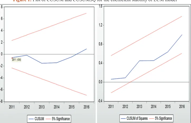
heteroscedasticity. Stability test is conducting using the cumulative
sum of recursive residuals (CUSUM) and the cumulative sum of square recursive residuals (CUSUMSQ) suggested by Brown et al. (1975). If the plots of CUSUM and CUSUMSQ are within the critical bounds in 5% level of significance, the null hypothesis
that all coefficients on regression model are stable cannot be
rejected. Thus, when the error correction model of ARDL bounds are estimated, Pesaran and Pesaran (1997) suggest the application of the cumulative sum of recursive residuals (CUSUM) and the cumulative sum of square recursive residuals (CUSUMSQ) to assess for parameters’ stability.
5. EMPIRICAL RESULTS AND DISCUSSION
5.1. Unit Root TestsBefore employing ARDL Bounds testing, we examine variables’
stationarity in order to determine their integration order. In this
way, we ensure that series are not integrated order two I(2),
avoiding incorrect results on the following estimations. The presence of variables integrated order two lead to the invalidity
of F statistics suggested by Pesaran et al. (2001). The hypotheses for variables’ integration on ARDL procedure refers that variables should be I(0) or I(1) Pesaran et al. (2001). For this reason, we use Dickey-Fuller (1979; 1981), Phillips-Peron (1988) and Kwiatkowski et al. - KPSS (1992) tests. The results of these unit
root tests are presented on Table 1.
The results on Table 1 show that series are integrated I(0) and I(1). Because the sample size is small, the ARDL test must be used for
cointegration of the variables.
5.2. Bounds Tests for Cointegration
It was referred previously on section 4.2.1, in the second stage, before
estimating the models on equations (13), (14), (15), (16) and (17) with ARDL method, that it is necessary to find the number of time lags of the variables’ model using the corresponding criteria. The lag length for each variable on ARDL model is important, because the error term
should avoid non-normality, autocorrelation and heteroscedasticity.
For the number of time lags we used Akaike criterion (AIC criteria).
On the following Table 2, the results are presented of the ARDL bounds test. Critical bounds derive from Narayan’s paper (2005)
which are more appropriate for small sample.
According to Narayan (2005), the existing critical values reported in Pesaran et al. (2001) cannot be used for small sample sizes because they are based on large sample sizes. Narayan (2005) provides a set of critical values for sample sizes ranging from 27 observations. They are 2.68-3.53 at 90%, 3.05-3.97 at 95%, and
3.81-4.92 at 99%.
The results of the Table 2 show that we get five cointegrating
vectors. So, we can see that there is a long run relationship among
5.3. Estimated Long Run Coefficients using the ARDL
Approach
After the confirmation of long run relationship among the variables the next step is to determine the short and long run elasticity. The
results on these dynamics are presented on Table 3.
X2N, X2SC, and X2ARCH are normality (Jarque-Bera), Lagrange
multiplier values for serial correlation), and ARCH tests for
heteroscedasticity.
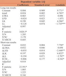
The results of Table 3 show that market openness and capital have positive effect in the economic growth of Poland whereas
financial development and labor seems to be correlated
negative. Because capital variables and labor are statistical significant in 1% and 10% level of significance, we can say
that 1% capital increase will cause increase in development by
0.20% approximately while a labor increase by 1% will affect development negatively by 0.13% approximately. This result is in accordance with Kosztowniak (2013) paper which claims that
the real important factor for economic growth is gross domestic
expenditures of fixed capital.
The short run results on Table 3 show that the short run coefficient on error correction term is −0.806 and statistical significant in 1% level of significance. That implies that there is a long run relationship among variables for Poland. Moreover, this result shows that the short-run change from the long-run equilibrium is corrected by 80.6% each year. The results from short run analysis are similar to those coming from long run. Market openness
and capital have positive effect in economic growth whereas
financial growth and labor are negative. Also, labor and capital are statistical significant in 1% level of significance. Finally,
diagnostic tests, both in the short and long run satisfy all the
Table 1: Unit root tests
Var. ADF P-P KPSS
C C, T C C,T C C, T
Levels
LQ 0.258 (0) −1.869 (1) 0.180[1] −3.659[3]** 0.769[3] 0.098[2]*
LTRA −1.870 (0) −1.325 (0) −1.997[2] −1.325[0] 0.765[3] 0.179[3]***
LFD −0.303 (0) −3.121 (1) −0.278[3] −2.430[2] 0.723[3]*** 0.118[2]***
LK −0.680 (5) −5.459 (4)* −0.526[0] −2.644[2] 0.718[3]*** 0.085[2]*
LL −0.109 (0) −2.490 (0) −0.589[3] −2.490[0] 0.461[3]** 0.184[3]***
First differences
ΔLQ −6.989 (0)* −3.788 (5)** −6.989[0]* −7.892[5]* 0.132[1]* 0.114[2]*
ΔLTRA −4.763 (0)* −5.210 (0)* −4.763[1]* −5.212[1]* 0.340[1]* 0.052[1]*
ΔLFD −4.369 (1)* −4.273 (1)** −4.023[7]* −3.941[7]** 0.103[3]* 0.082[4]*
ΔLK −4.604 (4)* −4.319 (4)* −3.806[5]* −4.598[8]* 0.093[0]* 0.096[0]*
ΔLL −4.549 (0)* −4.166 (0)** −3.490[1]** −4.161[1]** 0.426[3]** 0.184[2]***
*, ** and ***show significant at 1%, 5% and 10% levels respectively. The numbers within parentheses followed by ADF statistics represent the lag length of the dependent variable used to obtain white noise residuals. The lag lengths for ADF equation were selected using Schwarz information criterion (SIC). Mackinnon (1996) critical value for rejection of hypothesis of unit root applied. The numbers within brackets followed by PP and KPSS statistics represent the bandwidth selected based on Newey and West (1994) method using Bartlett Kernel. C=Constant, T=Trend, L=log, Δ=First differences
Table 2: The ARDL bounds testing cointegration approach analysis
Bounds testing to cointegration Diagnostic tests
Estimated models Optimal lag length F-statistics Jarque-Bera ARCH (1) RESET LM (1)
FQ (Q/TRA, FD, K, L) (1,3,3,3,3) 8.211* 11.48* 0.236 0.062 4.023
FTRA (TRA/Q, FD, K, L) (2,2,3,1,3) 7.515* 0.986 0.025 0.015 12.83*
FFD (FD/TRA, Q, K, L) (2,2,3,2,2) 11.36* 1.273 0.323 1.893 10.80*
FK (K/TRA, FD, Q, L) (1,2,2,0,0) 9.675* 1.119 0.172 0.798 0.170
FL (L/TRA, FD, K, Q) (3,3,3,3,2) 9.019* 0.825 3.445** 0.688 10.79*
*, **, ***represent significance at 1, 5, 10% levels respectively. Appropriate lag length of the variables is selected following AIC
Table 3: ARDL long-run and short-run results
Dependent variable: LQ
Coefficients Standard error t-statistic Long-run results
Constant 8.884 0.909 9.771*
trend 0.024 0.005 4.703*
LTRA 0.065 0.072 0.896
LFD −0.024 0.023 −1.071
LK 0.198 0.045 4.386*
LL −0.128 0.074 −1.735***
Adjusted
R2 0.997
F-statistic 1820.5* X2N 1.285
X2SC 3.178
X2ARCH 0.685
Short-run results
Constant 0.032 0.004 7.758*
ΔLTRA 0.032 0.046 0.694
ΔLFD −0.035 0.014 −2.448**
ΔLK 0.197 0.028 6.822*
ΔLL −0.194 0.071 −2.707*
ECMt−1 −0.806 0.177 −4.542*
Adjusted
R2 0.818
F-statistic 23.591*
X2N 1.085
X2SC 1.223
X2ARCH 0.166
assumptions of the linear regression model where autocorrelation and heteroscedasticity are absent and residuals are normally distributed.
5.4. Stability Test
Diagnostics tests on the results on Table 3 shown that both in long
run estimation of ARDL model and also on short run estimation
all hypotheses of linear regression model are valid. The stability
of long run coefficients is tested from short run dynamics of the
model. On the error correction model presented on Table 3, the
cumulative sum of recursive residuals (CUSUM) and the CUSUM of square residuals (CUSUMSQ) are applied in order to evaluate parameters’ stability. If the plot of CUSUM and CUSUMSQ are within the critical bounds on 5% level of significance, this means
that the model is stable. On Figure 1, the results on CUSUM and CUSUMSQ are shown.
The results on the above figure confirm the long run relationships among variables. Also, the absence of instability of the coefficients is also clear and this is evident from the plot of CUSUM και CUSUMSQ statistics which fall inside the critical bounds of the 5% confidence interval of parameter stability.
6. DISCUSSION AND CONCLUSION
Market openness promotes economic growth through various
channels such as attracting foreign direct investment, accessing advanced technology to boost domestic production, and enhancing productivity. In theoretical literature and empirical research there
are many different explanations for the role and implications of market openness in host countries. Other works show a positive
impact on economic growth, while others have come to different results. However, in all of them there is a broad consensus regarding the assertion that the increase in productivity is necessary for creating wealth and improving the competitiveness of a country.
Cobb-Douglas production function is considered a useful and
powerful tool for macroeconomic analysis and valuation of structural policies because it is often used for the analysis of
the profit and the measurement of manpower of a country. This functional form, however, requires some acceptances especially on
the functional form of the production technology on characteristics
of the technological progress, as well as markets’ function.
This paper examines whether market openness and financial sector promotes or hampers economic growth in Poland in the long run. For this purpose, we used the Cobb-Douglas production function as formulated by Mankiw et al. (1992). The paper was carried out for the period 1990-2016 and the recently developed econometric ARDL cointegration technique was used for the long-term equilibrium relationship of the time series of the model.
Furthermore, for stability of parameters on the error correction
model the cumulative sum of residuals (CUSUM) and cumulative sum of squared residuals (CUSUMSQ) suggested by Brown et al. (1975) was used.
The results of the paper have shown that long-term market openness and capital have a positive impact on Poland’s economic growth, while financial development and labor appear to be negatively
related. This result is partly in line with the study conducted by
Kosztowniak (2013) which argues that the really important factor
for increasing economic growth is the gross domestic expenditure on fixed capital. Also, the results of the short-term analysis are similar to those of the long-term. Market openness and capital
have a positive effect on economic growth, while the effect of
financial growth and labor is negative.
To sum up, we can presume that during the examined period,
capital seems to be an impetus for economic growth both in the
short and long run. Market openness contributes to the mobility
resources from developed to developing economies with the help
of technological progress. Also, market openness allows foreign
direct investment in host country to contribute in supplementing
domestic capital and redefining economic efficiency with the
increase of productivity. In spite of this, the results of this paper
shown that even if market openness is positive towards growth in the short and long run, it is not statistical significant on both
regressions. So, the conclusion of the paper is in accordance
with the paper of Kosztowniak (2013) which claims that the
most important factor for the increase of economic growth is
the gross domestic expenditure of fixed capital and not foreign direct investment through market openness. The negative sign of financial development possibly is owed to the poor organization of financial sector of Poland which explains the negative sign and it is statistical significant in the short run estimation of the model.
Finally, the negative sign that labor gets on economic growth is due to the recent world crisis, where most of the countries faced problems on employment. However, for the less developed countries low levels of employment, low levels of wages and insecure employment was considered a continuous problem.
As Kosztowniak (2013) referred to her paper, the recession on 2001-2002 in European Union affected also the Central Europe countries. This resulted in an instability of inflows and outflows of foreign direct investment on Poland giving the negative sign to employment on country’s productivity.
REFERENCES
Barro, R. (2003), Determinants of economic growth in a panel of countries. Annals of Economics and Finance, 4, 231-274.
Brown, R.L., Durbin, J., Evans, J.M. (1975), Techniques for testing the constancy of regression relations over time. Journal of the Royal Statistical Society, 37, 149-163.
Cobb, C.W., Douglas, P.H. (1928), A theory of production. American Economic Review, 18(1), 139-165.
Das, A., Paul, B.P. (2011), Openness and growth in emerging Asian economies: Evidence from GMM estimation of a dynamic panel. Economics Bulletin, 31, 2219-2228.
Dickey, D.A, Fuller, W.A. (1981), Likelihood ratio statistics for autoregressive time series with a unit root. Econometrica, 49(4), 1057-1072.
Dickey, D.A., Fuller, W.A. (1979), Distributions of the estimators for autoregressive time series with a unit root. Journal of American Statistical Association, 74(366), 427-431.
Economidou, C., Murshid, A.P. (2008), Testing the linkages between trade and productivity growth. Review of Development Economics, 12, 845-860.
Greenaway, D., Morgan, C.W., Wright, P.W. (2002), Trade liberalisation and growth: New methods, new evidence. Journal of Development Economics, 67, 229-244.
Grossman, G.M., Helpman, E. (1990), Comparative advantage and long-run growth. American Economic Review, 80, 796-815.
Jenkins, H.P., Katircioglu, S.T. (2010), The bounds test approach for cointegration and causality between financial development,
international trade and economic growth: the case of Cyprus. Applied Economics, 42, 1699-1707.
Johansen, S. (1988), Statistical analysis of cointegration vectors. Economic Dynamic Control, 12, 231-254.
Kosztowniak, A. (2013), Foreign direct investment as a factor of economic growth in Poland. Empirical analysis for the period 1995-2012. Advances in Economics and Business, 1(2), 203-212.
Kosztowniak, A. (2014), Analysis of the cobb-douglas production function as a tool to investigate the impact of FDI net inflows on gross domestic product value in Poland in the period 1994-2012. Oeconomia Copernicana, 5(4), 169-190.
Krueger, A.O. (1978), Foreign Trade Regimes and Economic Development: Liberalization Attempts and Consequences. Cambridge, MA: Ballinger.
Kwiatkowski, D., Phillips, P.C., Schmidt, P., Shin, Y. (1992), Testing the null hypothesis of stationarity against the alternative of a unit root. Journal of Econometrics, 54, 159-178.
MacKinnon, J.G. (1996), Numerical distribution functions for unit root and cointegration tests. Journal of Applied Econometrics, 11(6), 601-618.
Mankiw, N.G., Romer, D., Weil, D.N. (1992), A contribution to the empirics of economic growth. Quarterly Journal of Economics, 107, 407-437.
Narayan, P.K. (2005), The savings and investment nexus for China: Evidence from cointegration tests. Applied Economics, 37, 1979-1990.
Newey, W.K., West, K.D. (1994), Automatic lag selection in covariance matrix estimation. Review of Economic Studies, 61(4), 631-654. Nishimizu, M., Robinson, S. (1984), Trade policies and productivity
change in semi industrialized countries. Journal of Development Economics, 30, 93-102.
Pesaran H.M., Shin, Y. (1999), Autoregressive distributed lag modelling approach to cointegration analysis. In: Storm, S., editors. Econometrics and Economic Theory in the 20th Century: The Ragnar
Frisch Centennial Symposium. Ch. 11. Cambridge: Cambridge University Press.
Pesaran, M.H., Shin, Y., Smith, R.J. (2001), Bounds testing approaches to the analysis of long run relationships. Journal of Applied Econometrics, 16, 289-326.
Phillips, P.C.B., Perron, P. (1988), Testing for a unit root in time series regression. Biometrika, 75, 335-346.
Pradhan, R.P., Arvin, M.B., Norman, N.R., Hall, J.H. (2015), A quantitative assessment of the trade openness economic growth nexus in India. International Journal of Commerce and Management, 25(3), 267-293.
Romer, P.M. (1990), The problem of development: A conference of the institute for the study of free enterprise system. Journal of Political Economy, 98, 1-11.
Shahbaz, M. (2012), Does trade openness affect long run growth? Cointegration, causality and forecast error variance decomposition tests for Pakistan. Economic Modelling, 29(6), 2325-2339. Tyler, W.J. (1981), Growth and exports expansion in developing