Power System Fault Detection Using Conductor Dynamics

University of New Orleans University of New Orleans

ScholarWorks@UNO

ScholarWorks@UNO

University of New Orleans Theses and

Dissertations Dissertations and Theses

8-10-2005

Power System Fault Detection Using Conductor Dynamics

Power System Fault Detection Using Conductor Dynamics

Jeff Dicharry

University of New Orleans

Follow this and additional works at: https://scholarworks.uno.edu/td

Recommended Citation Recommended Citation

Dicharry, Jeff, "Power System Fault Detection Using Conductor Dynamics" (2005). University of New Orleans Theses and Dissertations. 289.

https://scholarworks.uno.edu/td/289

POWER SYSTEM FAULT DETECTION USING CONDUCTOR DYNAMICS

A Thesis

Submitted to the Graduate Faculty of the University of New Orleans in partial fulfillment of the requirements for the degree of

Master of Science in

The Department of Electrical Engineering

by

Jeff Dicharry

B.S.E.E. Louisiana State University, 2000

Acknowledgement

The research presented in this paper could not have been possible without the hard

work and patience of the professors at the University of New Orleans. The quality of education

provided for my degree is a reflection of the knowledge and willingness of the instructors. I

would especially like to thank the members of my thesis committee, Henri A. Alciatore, M.S.,

Edit J. Bourgeois, Ph.D., and Vesselin Jilkov, Ph.D.

I would also like to recognize my co-workers at Entergy Services, Inc. for their willingness

to teach me about substation design and the power industry. I would like to thank Tammy

Lapeyrouse for giving me the opportunity to be employed as a substation designer at Entergy and

involved with the IEEE substations committee. The experiences I gained from employment and

the IEEE have proved beneficial in my educational degree and professional career.

I would like to thank my parents, Joseph M. Dicharry and Maureen C. Dicharry, whose

encouragement and belief in me are responsible for my successes in life.

Finally, I would like to thank Rebecca D. Schneider for her support and patience

Table of Contents

List of Figures ... v

List of Tables ... ix

Abstract ... x

1.0 Introduction... 1

1.1 Motivation for Research ... 5

1.2 Objectives of Study ... 5

1.3 Outline of Topics Covered... 5

2.0 Power System Fault Currents... 7

2.1 Derivation of Fault Current Components ... 7

2.2 Analysis of Fault Current Components ... 10

2.3 Types of Power System Faults ... 13

3.0 Fault Current Forces... 17

3.1 Electromagnetic Conductor Forces ... 17

3.2 Three Phase Electromagnetic Conductor Forces ... 24

3.3 Single Conductor Three Phase Rigid Bus... 26

3.4 Bundled Conductor Three Phase Rigid Bus ... 28

4.0 Substation Bus Response... 32

4.1 Static Analysis of Rigid Bus Mechanical Response ... 32

4.2 Dynamic Analysis of Rigid Bus Mechanical Response ... 35

4.3 Dynamic Response of Bundled Conductor Faults ... 47

5.0 Optical Method of Fault Detection... 52

5.1 Physical Configuration ... 52

5.2 Time-Current Coordination ... 54

5.3 Multiple Circuit Detection Coordination... 62

6.0 Conclusions and Further Research... 65

6.1 Suggestions for Further Research ... 66

Appendix B: Bus Dynamic Fault Detector Design Flowchart ... 87

References ... 88

List of Figures

Figure 1.1: Typical Relay Time-Overcurrent Curves ... 2

Figure 1.2: Typical Relay and Damage Time-Overcurrent Curves... 3

Figure 1.3: Typical Relay and Damage Time-Overcurrent Curves w/ Backup Relays ... 4

Figure 2.l: Circuit Model for Power System Fault Analysis ... 7

Figure 2.2: Fault Current Including Transient Component ... 10

Figure 2.3: Transient Fault Current Component Based on X/R Ratio... 11

Figure 2.4: Frequency Components of Fault Current ... 12

Figure 2.5: Example of B-Phase to Ground Fault Current... 13

Figure 2.6: Example of A-B Phase Fault Current... 14

Figure 2.7: Example of A-B Phase to Ground Fault Current ... 15

Figure 2.8: Example of Three Phase Fault Current ... 16

Figure 3.1: Parallel Conductor Forces ... 18

Figure 3.2: Input Currents 120 Degrees Out of Phase ... 19

Figure 3.3: Electromagnetic Force Fab(t) ... 20

Figure 3.4: Frequency Content of Force Fab(t) ... 21

Figure 3.5: Input Currents 120 Degrees Out of Phase with Transients ... 22

Figure 3.6: Electromagnetic Force Fab(t) with Transients ... 23

Figure 3.7: Frequency Content of Force Fab(t) with Transients ... 23

Figure 3.8: Example of Substation Three Phase Rigid Bus ... 24

Figure 3.9: Three Phase Fault Current Force Vectors... 25

Figure 3.11: Bundled Fault Current Force Vectors ... 29

Figure 4.1: Beam Deflection Due to an Evenly Distributed Load... 33

Figure 4.2: Example of a Single Bus Span with Two Structures ... 34

Figure 4.3: Example of a Single Bus Span with Bundled Rigid Conductors... 34

Figure 4.4: Spring-Mass System Representation of a Rigid Bus Span... 35

Figure 4.5: Magnification Factor of a Spring-Mass System ... 37

Figure 4.6: Frequency Response of a Spring-Mass System ... 39

Figure 4.7: Natural Frequencies for Several Conductor Types ... 41

Figure 4.8: Spring-Mass System Representation of a Rigid Bus Span with Insulators.... 42

Figure 4.9: Electrical Equivalent Model of a Mechanical Spring-Mass System... 43

Figure 4.10: Natural Frequencies of a Dual Spring-Mass System ... 44

Figure 4.11: Transient Step Response of a Dual Spring-Mass System... 45

Figure 4.12: Bundled Conductor Displacement Due to Fault Forces... 47

Figure 4.13: Bundled Conductor Short Circuit Forces ... 48

Figure 4.14: Transient Bundled Conductor Short Circuit Forces... 50

Figure 4.15: Average Bundled Conductor Short Circuit Forces ... 51

Figure 5.1: Physical Fault Detection Configuration ... 53

Figure 5.2: Electrical Diagram of Detection Logic ... 55

Figure 5.3: Profile View of Physical Fault Detection Configuration ... 56

Figure 5.4: Conductor Displacement with Reflecting Mirror Position... 57

Figure 5.5: Deflection Displacement Detection Pulses... 57

Figure 5.8: Displacement of Conductor Bundles... 61

Figure 5.9: Fault Current Contributions for Fault on Circuit 1 ... 62

Figure 5.10: Fault Current Contributions for Fault on Circuit 2 ... 63

Figure 5.11: Fault Current Contributions for Fault on Circuit 3 ... 63

Figure 5.12: Fault Current Contributions for Fault on Circuit 4 ... 64

Figure A.1: Appendix A RMS Power System Electrical Oneline ... 67

Figure A.2: Phase to Ground Fault Current... 69

Figure A.3: Three Phase Fault Current ... 70

Figure A.4: A Phase to Ground Fault Current Forces... 71

Figure A.5: A to B Phase Fault Current Forces... 71

Figure A.6: A to B Phase to Ground Fault Current Forces ... 72

Figure A.7: A to C Phase Fault Current Forces... 72

Figure A.8: A to C Phase to Ground Fault Currernt Forces... 73

Figure A.9: Three Phase Fault Current Forces ... 73

Figure A.10: Primary Overcurrent Relay Settings... 76

Figure A.11: Conductor Deflection Using Primary Relaying ... 77

Figure A.12: Pulse Width Using Primary Relaying... 77

Figure A.13: A Phase to Ground Fault Conductor Displacements... 79

Figure A.14: A Phase to Ground Fault Conductor Deflection Detector Pulses ... 79

Figure A.15: A to B Phase Fault Conductor Displacements ... 80

Figure A.16: A to B Phase Fault Deflection Detector Pulses... 80

Figure A.17: A to B Phase to Ground Fault Conductor Displacements ... 81

Figure A.19: A to C Phase Fault Conductor Displacements ... 82

Figure A.20: A to C Phase Fault Deflection Detector Pulses... 82

Figure A.21: A to C Phase to Phase Fault Conductor Displacements ... 83

Figure A.22: A to C Phase to Ground Fault ... 83

Figure A.23: Three Phase Fault A and D Bundle Conductor Displacements ... 84

Figure A.24: Three Phase Fault A and D Bundle Deflection Detector Pulses ... 84

Figure A.25: Three Phase Fault B and E Bundle Conductor Displacements ... 85

Figure A.26: Three Phase Fault B and E Bundle Deflection Detector Pulses ... 85

Figure A.27: Three Phase Fault C and F Bundle Conductor Displacements ... 86

Figure A.28: Three Phase Fault C and F Bundle Deflection Detector Pulses... 86

List of Tables

Table 5.1: Fault Current Contributions for Various Faulted Circuits ... 64

Table A.1: Appendix A Fault Current Values ... 68

Table A.2: 8A-67971A 230kV Insulator Mechanical Specifications ... 74

Abstract

Power system fault detection is conventionally achieved using current and potential

measurements. An alternate and unconventional form of protective relaying is feasible using

rigid bus conductor motion as the means of detection. The research presented focuses on the

detection of power system faults using visual displacement of conductor spans. Substation rigid

bus conductor motion is modeled using dual spring-mass systems for accurate representation of

conductor response to electromagnetic forces generated during system faults. Bundled rigid

conductors have advantages including detection independent of system load currents and

improved ability to detect polyphase and single phase faults. The dynamic motion of the

conductors during the fault is optically monitored with a laser detection system.

Time-overcurrent characteristics are derived for the application of fault detection. The response time

of the conductor detector system is slower than conventional relays due to the natural

frequencies of the conductor span limiting the speed of its displacement. This response time

makes the fault detection system using conductor displacement an ideal candidate for a backup

1.0 Introduction

Protective relaying in power systems is crucial to safety and reliability. From the simple

household fuse to high voltage transmission line breakers, the purpose of the protective devices

is to interrupt flow effectively. This interruption results from a three step process: detect, decide,

and act.

Typical power system protective relays utilize electromechanical or microprocessor

technology to perform the three step process. Based on relay settings, the relay can detect the

fault and make a decision to trip a protective device. If the decision is made to trip, the action is

performed using a trip signal output from the relay and the circuit is opened. The critical inputs

to the protective relay are current and potential transformers connected to the monitored power

system element.

A properly protected power system has several relays with overlapping zones of

protection. The primary purpose of this is to provide adequate backup protection in the event of

improper operation. Relay settings including time and overcurrent relationships ensure proper

coordination with overlapping zones. Backup relays within the same zone provide additional

security, but often rely on the same source of electrical power and current or potential

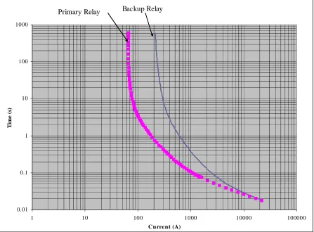
transformers. This does, however, provide a margin of security for improperly set relays. Figure

0.01 0.1 1 10 100 1000

1 10 100 1000 10000 100000

C urrent (A)

Ti

m

e

(s)

Primary Relay Backup Relay

Figure 1.1: Typical Relay Time-Overcurrent Curves

Inspection of figure 1.1 indicates primary relays are designed to trip before backup

relays. This is based on higher current for a shorter period of time. Typically, these values are

only attained during system faults. In the event that the primary relay does not operate as

planned, the backup relay will trip with some time delay. Overlapping zones of protection also

have similar time-overcurrent coordination curves.

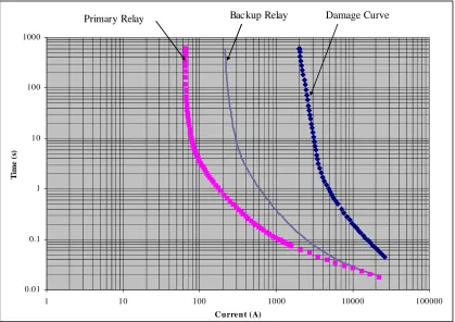
Figure 1.2 includes the location of a typical power system device damage curve. It is

imperative that protective devices act prior to the damage curve or the relays will provide

inadequate protection. If the magnitude and duration of fault currents violate the damage curve,

increases stress upon utility budgets with influence on customer rate bases. Replacement or

repair of such equipment is difficult due to the physical size and availability. Any way to avoid

equipment damage should be utilized to minimize these negative effects.

0.01 0.1 1 10 100 1000

1 10 100 1000 10000 100000

C urren t (A)

Ti

m

e

(s)

Primary Relay Backup Relay Damage Curve

Figure 1.2: Typical Relay and Damage Time-Overcurrent Curves

Figure 1.3 depicts a second backup relay. This type of protection acts similar to an

overcurrent relay with time delay or a differential relay with time delay. When the current

reaches the set level, sends an instantaneous trip signal. The location of the line is determined

based on relay coordination with proper settings. The redundant backups serve as an extra layer

0.01 0.1 1 10 100 1000

1 10 100 1000 10000 100000

C u rre nt (A)

T

im

e (

s)

Primary Relay Backup Relay Damage Curve Backup Relay #2

Figure 1.3: Typical Relay and Damage Time-Overcurrent Curve with Backup Relays

The intention of the research presented in this document is to present a method of backup

relay protection similar to the backup relay #2 depicted in figure 1.3. Through detailed analysis,

the novel application of conductor dynamics will be used for the purpose of fault detection. This

will be accomplished without the use of conventional equipment including electromechanical

relays, microprocessor relays, potential transformers, and current transformers. Through

deflection calculations and varied design parameters, the motion of rigid bus conductors can

provide visual indication of a power system fault and is capable of being integrated on the

1.1 Motivation for Research

The use of a new method of power system fault detection serves as backup protection

device with relatively low construction and maintenance costs. While the emphasis of the

research presented in this thesis is focused upon the application to power systems inside medium

to high voltage substations, the information presented can be applied in a variety of electrical

applications at various voltage levels.

1.2 Objectives of Study

The primary objective of the research presented in this paper is to provide design details

and analysis methodology for a substation design engineer to design a section of substation rigid

bus for the purpose of fault detection through visual indication.

A secondary objective to the research presented is to reveal the advantages of bundled

rigid bus in the application of fault detection using conductor dynamics.

While the design and dynamic response of substation rigid bus inside substations has

been widely studied, the research focuses on the use of dynamic analysis for bus spans [2].

Static analysis was not chosen for this research due to its limitations for the application of the

transient dynamic response.

1.3 Outline of Topics Covered

Section 2 includes the details and derivations of the transient nature of several types of

power system faults. The information presented will be used to provide an accurate dynamic

Section 3 describes the dynamic motion of the bus based on deflection characteristics and

its application to rigid bus. This section also presents limitations to conventional three phase bus

configurations for its use in fault detection and lists advantages for bundled conductors.

Section 4 focuses on the dynamic analysis of bundled substation rigid bus and its analogy

to the dual spring-mass mechanical system. Emphasis is placed on natural frequencies and

variations of span components.

Section 5 describes the calibration and determination of relay settings in relay

coordination. The method chosen to detect faults uses an optical system configuration for visual

deflection indication.

Appendix A provides a detailed example of the use of conductor dynamics for the

purpose of fault detection.

Appendix B contains a flowchart to be utilized for the design of conductor bus spans to

effectively detect fault currents based on displacement. It is a practical guide for the substation

2.0 Power System Fault Currents

Power system fault current analysis is an extensive portion of power engineering. Entire

textbooks have been written describing methodology for the detailed analysis of power system

faults. This section briefly summarizes the transient and steady state portion of fault currents.

Both of these components are necessary for the proper dynamic analysis of the substation bus

during fault conditions.

2.1 Derivation of Fault Current Components

A detailed derivation of fault current components is given in [3]. The components

derived are the steady state and transient portions of fault currents and should not be confused

with the method of symmetrical components for fault current analysis in unbalanced systems [1].

The information derived in [3] is summarized in this section.

R

L

Load

e(t)

Fault

Location

i(t)

The voltage source in figure 2.1 is defined in equation 2.1. The source is sinusoidal with

system frequency ( ), RMS voltage magnitude (V), and phase angle (φ).

) t cos( V 2

e(t)= ω +φ (2.1)

Analysis of the circuit in figure 2.1 with shorted load during a fault using Kirchhoff’s

voltage law yields equation 2.2.

dt di(t) L i(t) R

e(t)= + (2.2)

The use of the Laplace transform and solving for i(t) assuming initial current i(0)=c in

equation 2.2 is shown in equation 2.3. N(s) is defined as the Laplace transform of cos(wt+ø).

c sL R L N(s) sL R V 2 i(s) + + + = (2.3)

The inverse Laplace transform of equation 2.3 yields:

∫

+

= − t − −

0 ) (t L R t L R )d cos( e L V 2 e c

This is further evaluated by expansion of the integral to equation 2.5: )) t sin( L ) t cos( (R L w R V 2 i(t) 2 2

2₊ ω +φ +ω ω +φ

= (2.5)

t L R t L R 2 2

2 _{w L} e (Rcos( t ) Lsin( )) ce

R V

2 − −

+ +

+ +

− ω φ ω φ

For ease of evaluation, variables and I are identified in equations 2.6 and 2.7.

R L )

tan(ξ =−ω (2.6)

2 2 2 L R V I ω +

= (2.7)

Substitution of equations 2.6 and 2.7 into 2.5 is shown in equation 2.8.

t L R )]e cos( I 2 [c ) t cos( I 2

i(t)= ω +φ+ + − φ+ − (2.8)

Inspection of equation 2.8 reveals both the steady state (equation 2.9) and transient

(equation 2.10) components of the fault current.

) cos(wt

I 2

i(t)_steadystate = +φ + (2.9)

] e )) cos( I 2 [c i(t) t L R transient − + −

2.2 Analysis of Fault Current Components

The steady state fault current in equation 2.9 is commonly referred to in the power

industry as the fault current at a particular location. The introduction of the transient portion of

fault current in equation 2.10 shows the first several cycles of the fault current can be much

higher than the value of steady state current. This neglects initial current and assumes φ=- .

Figure 2.2 depicts this scenario using a 60Hz frequency.

0 0.02 0.04 0.06 0.08 0.1 0.12 0.14 0.16 0.18 -1.5

-1 -0.5 0 0.5 1 1.5 2 2.5

Time (s)

C

urr

ent

(A

m

ps

)

Transisent + Steady State Components Transient Component

Figure 2.2: Fault Current Including Transient Component

The transient fault current is a function of the system resistance and reactance. The ratio

of this reactance and resistance is commonly referred to as the X/R ratio of the power system.

0 0.05 0.1 0.15 0.2 0.25 0.3 0.35 0

0.5 1 1.5

Time (s)

C

ur

ren

t

(A

mps

)

X/R=5 X/R=10 X/R=15 X/R=20 X/R=25 X/R=30 X/R=35

Figure 2.3: Transient Fault Component Based on System X/R Ratio

Inspection of figure 2.3 and equation 2.10 indicates that the magnitude of the fault current

transient component is the same at the initiation of the fault for any X/R ratio. It decays slower

with a higher X/R ratio than a low one. The response of the bus to the system fault current and

its generated forces is a function of this X/R ratio.

The X/R ratio is a function of fault location. A fault near a transformer generally has a

high X/R ratio due to the windings of the transformer and its impact in increasing the reactance

at the fault location. This increased reactance will slow the transient decay time in comparison

with a low voltage distribution feeder with a smaller X/R ratio and shorter decay time. Any use

of protective relaying should consider this X/R ratio for the instantaneous and transient fault

The frequency components of fault currents including transient components can be

attained using Fourier analysis. The primary frequencies are 60Hz with a DC component.

Figure 2.4 depicts the components for the first 11 msec of the time domain signal in figure 2.2.

The Fourier transform of the waveform of this time domain signal is defined as:

  

 

  

 

+ + +

+ =

L R

) cos( I

2 w) ( G

2 o 2

o φ _.

0 50 100 150 200 250 300 350 400 450 500

0 0.1 0.2 0.3 0.4 0.5 0.6 0.7 0.8 0.9 1

|G

(w)|

Frequency (Hz)

Transient + Steady State Fault Current

2.3 Types of Power System Faults

The four primary types of faults are detailed in [1]. These include phase to

ground, phase to phase, phase to phase to ground, and three phase. The use of symmetrical

component analysis described in [1] proves beneficial for calculation of each type of fault.

It is critical that the protection designed for the power system respond to each possible

fault condition. While the power system designer can account for several different types of

faults, the protective equipment may not be able to distinguish between the various types of

faults. An accurate system model for studying power system faults including correct system

impedance parameters will minimize calculated fault current errors.

An example of the B phase to ground fault is depicted in figure 2.5 using an X/R ratio of

15, fault current magnitude of 20kA RMS, and load current of 2kA RMS. Symmetry of

approximately 120 degrees between phases is maintained through the fault duration.

0 0.02 0.04 0.06 0.08 0.1 0.12 0.14 0.16 0.18 -3

-2 -1 0 1 2 3 4 5x 10

4

Time (s)

C

ur

re

nt

(A

m

ps

)

A phase B phase C phase

An example of a phase to phase fault is shown in figure 2.6. The same assumptions used

in figure 2.5 have been used for depiction of the fault. Because the fault current does not include

a ground path, the two faulted phases are symmetric in steady state magnitude as indicated in [6].

While the transient component is shown as identical for both phases, the transient portion of each

phase may not actually be identical as indicated in [2]. The phase angle of the C phase current

relative to A phase is a function of system topology and varies with system locations.

0 0.02 0.04 0.06 0.08 0.1 0.12 0.14 0.16 0.18 -3

-2 -1 0 1 2 3 4 5 6x 10

4

Time (s)

C

urr

ent

(A

m

ps

)

A phase B phase C phase

Figure 2.6: Example of A to B Phase Fault Current

The introduction of the ground path in the phase to phase fault depicted in figure 2.6

removes the symmetry of the faulted phases as indicated in figure 2.7 using the same

assumptions. Actual phase angles and transient component contributions will vary according to

0 0.02 0.04 0.06 0.08 0.1 0.12 0.14 0.16 0.18 -3

-2 -1 0 1 2 3 4 5 6x 10

4

Time (s)

C

ur

re

nt

(A

mps

)

A phase B phase C phase

Figure 2.7: Example of A to B Phase to Ground Fault Current

Three phase faults provide phase angles of approximately 120 degrees as indicated in

figure 2.8. Similar to phase to phase and phase to phase to ground faults, actual transient

components for faulted phases vary with system topology. The magnitudes of the faulted phase

currents are equal assuming a balanced three phase system. The introduction of the ground path

0 0.02 0.04 0.06 0.08 0.1 0.12 0.14 0.16 0.18 -3

-2 -1 0 1 2 3 4 5 6x 10

4

Time (s)

Cu

rre

nt

(A

m

p

s

)

A phase B phase C phase

Figure 2.8: Example of Three Phase Fault Current

The purpose of identifying the various types of system faults is to ensure the proposed

methods of relaying encompass all types of faults. The simple flow of too much current on an

electrical device can cause heat, flames, equipment damage, and lethal ground potential rise. A

protection scheme not encompassing every fault scenario provides additional risk to equipment,

3.0 Fault Current Forces

Extensive studies have been performed on substation rigid bus using various static and

dynamic models. This section describes methodology for both static and dynamic analysis of

fault current forces between rigid bus conductors. The conclusion is made that the dynamic

modeling of electromechanical forces provides a more accurate representation of actual forces

generated than static forces.

3.1 Electromagnetic Conductor Forces

The magnetic force on a current carrying wire is detailed in [7]. The equations used in

this section are primarily obtained from [7] with application to the motion of bus relevant to fault

current response.

The force vector due to electromagnetism on a conductor is defined in equation 3.1. The

force is dependent upon the conductor length, magnetic field generated, and applied current.

B L i

F v v

v

⊗

= (3.1)

Equation 3.1 applied to the scenario of two parallel conductors depicted in figure 3.1

yields a cross product which can be reduced to equation 3.2, based on the parallel nature of the

design.

cos(0) B

L i

F_ab = _{b a} (3.2)

The magnetic field contribution from conductor A, Ba at wire B is defined in equation 3.3

where the permeability constant of air is _o = ×10−7and d is the distance between conductors.

d 2

i

Substitution of equation 3.3 into equation 3.2 with time varying input currents yields

equation 3.4. The output force vector is a function of time based on time and direction of the

input currents.

d 2

(t) i (t) i L (t)

F_ab o a b

v v v

= (3.4)

Two parallel conductors are depicted in figure 3.1. Currents are injected into the two

conductors with magnitudes vI_a(t)and vI_b(t). The direction convention of equation 3.4 is noted in

figure 3.1. The force on each conductor is identical in magnitude such that F_ab = F_ba .

Direction is dependent upon the direction of current as described in [7].

I

(t)

I

(t)

F

(t)

F

(t)

L

_d

Figure 3.1: Parallel Conductor Forces

If the currents vI_a(t)and vI_b(t)are in the same direction, the resulting force vector

(t)

Fv_ab produces a pinch effect where the two conductors are pulled together. On the contrary,

forces on conductors where AC currents produce dynamic forces with points of zero force at the

zero crossing of either input, vI_a(t)or vI_b(t).

In the electric utility, the use of static (DC) forces are not as common due to a primarily

AC dominated power grid. [1] explains the use of voltage vectors with their 120 degree phase

separation in the electric grid. Consider, for example, figure 3.1 with input currents separated

with a phase angle of 120 degrees as indicated in figure 3.2. This configuration is similar to two

phases of a distribution line without the presence of the third. The application of equation 3.4

with separation distance d = 1 ft and current magnitude of 1kA produces the dynamic force

(#/inch) as indicated in figure 3.3.

0 0.01 0.02 0.03 0.04 0.05 0.06 0.07 0.08 -1500

-1000 -500 0 500 1000 1500

Time (s)

Cu

rre

nt

(A

m

p

s

)

Ia(t) Ib(t)

0 0.01 0.02 0.03 0.04 0.05 0.06 0.07 0.08 -12

-10 -8 -6 -4 -2 0 2 4x 10

-3

Time (s)

F

a

b

(t)

(#

/i

n

)

Figure 3.3: Electromagnetic Force Fab(t)

Figure 3.3 shows a sinusoidal force with positive and negative portions at its force

frequency. This force frequency is twice that of the power frequency. A Fourier analysis of the

frequency content is shown in figure 3.4. For the case of the 60 Hz power frequency, the

frequency of force is 120Hz with a DC component. The Fourier transform is defined as:

    

  

+ +

= 1

d 2

I L G(w)

2 o 2 2

0 50 100 150 200 250 300 350 400 450 500 0

1 2 3 4 5 6x 10

-5

|G

(w)|

Frequency (Hz)

Frequency Content of Conductor Force

Figure 3.4: Frequency Content of Force Fab(t)

For comparative purposes, the use of equation 3.4 using the maximum magnitudes of the

input waveforms only (not the time varying portion) indicates a static force of approximately 4

times the dynamic force. This example shows the conservativeness nature of static analysis.

Dynamic analysis is more appropriate for situations which require accurate force calculations. A

conservative static value is industry accepted in [2] for calculations of bus structures designs.

For the application of fault detection using dynamics, this static analysis does not account for the

The presence of a transient component in fault current forces produces non-sinusoidal

force waveforms until the transient components decay. Figure 3.5 depicts the input current

waveforms of figure 3.2 including a transient portion with X/R = 15.

0 0.02 0.04 0.06 0.08 0.1 0.12 0.14 0.16 0.18 0.2 -1500 -1000 -500 0 500 1000 1500 2000 2500 3000 Time (s) Cu rre nt (A m p s ) Ia(t) Ib(t)

Figure 3.5: Input Currents 120 Degrees Out of Phase with Transients

Figure 3.6 shows the electromagnetic force waveform for the two currents presented in

figure 3.5. After the transient forces decay, the steady state waveform is identical to figure 3.3.

Its associated frequency spectrum for the first 11msec is shown in figure 3.7. The Fourier

transform is defined as:

        + +       + + = R ) cos( 1 2 1 d I L G(w) 2 2 2

0 0.02 0.04 0.06 0.08 0.1 0.12 0.14 0.16 0.18 0.2 -0.015

-0.01 -0.005 0 0.005 0.01 0.015 0.02 0.025

Time (s)

F

ab(

t)

(#/

in

)

Figure 3.6: Electromagnetic Force Fab(t) with Transients

0 50 100 150 200 250 300 350 400 450 500 0

0.2 0.4 0.6 0.8 1 1.2 1.4 1.6 1.8x 10

-4

|G(w

)|

Frequency (Hz)

Frequency Content of Conductor Force

During the decay, a 60Hz force contribution is present. A similar peak 120Hz force is

most apparent with contributions from a DC portion. Inspection of figure 3.6 indicate the first

several cycles more closely resemble a 60Hz waveform than a 120Hz one. The necessity for the

use of the transient 60Hz and DC component will become apparent on the discussion of bus

response in section 4.

3.2 Three Phase Electromagnetic Conductor Forces

The use of three phase electric systems is common throughout the power industry. The

infrastructure for the power grid particularly in substations and transmission lines, revolves

around construction of sets of three identical phases. Figure 3.8 depicts a typical substation bus

with insulator supports1.

Aluminum Tube Rigid Bus

Insulator

Support Structure

Figure 3.8 depicts a single support structure to which three station post insulators are

attached. The insulators are in line to support rigid bus tubing using a bus clamp. Multiple spans

of bus are used to carry current to electrical devices inside the substation. The substation

designer has the flexibility to utilize multiple structures, insulators, and busbar according to

electrical and physical constraints for the construction of substation bus. Figure 3.8 is one

possible configuration which should be analyzed in detail by the substation designer. Design

forces characterized for substation rigid bus in [2] include ampacity, corona, vibration,

gravitational, wind, fault current, expansion, insulator, and conductor.

The various forces acting on substation bus spans add as vectors. Figure 3.9 depicts the

net fault current forces for a plan view of a typical three phase span of bus. The forces are

depicted at different points along the conductor for clarity purposes; however, the forces actually

are evenly distributed on the bus as described in section 3.1.

F

(t)

Cø

F

(t)

Bø

F

(t)

Aø

F

(t)

F

(t)

F

(t)

Figure 3.9: Three Phase Fault Current Force Vectors

Assuming the positive X direction is from the A phase towards the C phase, the net force

(t) F (t) F (t)

Fv_A = v_AB +v_AC (3.5)

(t) F (t) F (t)

F_B v_AB v_BC

v

−

= (3.6)

(t) F (t) F (t)

F_C v_AC v_BC

v

− −

= (3.7)

3.3 Single Conductor Three Phase Rigid Bus

Due to the unpredictable nature of faults and their seemingly random phase selection, any

protection system should be able to detect any type of fault at any moment in time. This holds

true for optical detection based conductor deflection. The conductor must deflect noticeably for

any type of fault possible. Contributions from other phases have significant influence on this

deflection. This section discusses the electromagnetic force influences from each conductor

during the fault.

Inspection of equation 3.4 reveals a dependence upon the dynamic parameters of

(t)

I_a

v

and vI_b(t). For load current magnitudes much smaller than fault current magnitudes, the

force between phases is extremely small and can generally be neglected. Since these fault

current magnitudes are much higher than load currents, it is the scenario of a fault for which

forces become significant enough to move the bus and allow for visual fault detection.

The ratio of the static force produced in a phase to phase fault using equation 3.4 versus a

phase to ground fault is the ratio of fault current to load current of the unfaulted phase. Using

dynamic analysis, the ratio can be calculated as indicated in the example below. Due to the

unpredictable nature of faults, it is possible for a conductor to see significantly less force for a

B phase currents in equation 3.4 produces a large swing of possible fault current forces

dependent upon type of fault. This swing is significant enough to violate the stress limits on a

conductor or barely move a conductor during deflection.

For example, assume an A phase to ground fault and a A to B phase fault in a three phase

bus. The fault current is assumed to be 40kA RMS (steady state) and load current of 2kA RMS

in the unfaulted phases. Using equations 3.4 and 3.5 with 3 ft phase spacing and load current of

2000 amps on unfaulted phases, the time varying amplitude of the electromagnetic force on

phase A from phase B is depicted in figure 3.10. The influence of the C phase load current is

apparent on the magnitude of each peak of the waveform offset from the previous peak.

0 0.01 0.02 0.03 0.04 0.05 0.06

-0.4 -0.3 -0.2 -0.1 0 0.1 0.2 0.3 0.4

Time (s)

F

a

b

(t)

(#

/i

n

)

A Phase to Ground Fault A Phase to B Phase Fault

The static ratio of fault current force is 20. Dynamically at an instant in time, however,

the ratio is approximately 22. Inclusion of the ground path in the fault or a three phase fault

produces similar ratios. In either the static or dynamic analysis, it is clear in figure 3.10 that the

ratio of force generated can be large depending upon which type of fault occurs for a system.

3.4 Bundled Conductor Three Phase Rigid Bus

The use of bundled rigid conductors is generally not common in substations. Typically,

bundled conductors are used on transmission lines or jumper conductors which require additional

ampacity or to reduce the effects of audible corona on EHV substations. Conductor sizing is

generally based on heat rate for each installation (ampacity) and available hardware for the

conductors chosen. The rigid bus ampacity values from single conductors are usually sufficient

for heating due to load currents. The additional hardware and construction time are generally

unnecessary. Overall, the concept has not been utilized much inside the substation.

The use of bundled rigid conductors has a distinct advantage for fault detection purposes

which will be analyzed in this section and in section 4. These include conductor deflection

independent of unfaulted phase load current values or type of fault. Symmetry of the bundle

requires deflection of both phases to prevent false trips due to natural phenomenon such as

animal interference with the detection device.

As depicted in figure 3.10, the electromagnetic force differences from phase to phase and

phase to ground faults can be high. The deflection differences of each type of fault are

substantial enough to limit the detection of the fault depending upon conditions. Section 4 will

Equation 3.4 shows the dependence on load current in unfaulted phases to produce

electromagnetic forces. Thus, low load faults versus high load faults will produce different

forces on the conductors. Deflection of the bus is affected by this load current. A fault detection

system should be able to properly detect faults for any load level. This reality limits the use of

conventional three phase, single conductor bus designs.

Figure 3.11 depicts a plan view of the electromagnetic forces using a six conductor, three

phase bundled bus. As in figure 3.9, the forces are depicted at different points along the

conductor for clarity purposes; however, the forces actually are evenly distributed on the

conductors. It should be noted that phases A and D, B and E, C and F are equipotential and

bundled.

F_AB(t) Aø

F_AC(t)

F_AD(t)

F_AE(t)

F_AF(t)

F_DB(t) Dø

F_DC(t)

F_DE(t)

F_DF(t)

F_AD(t)

Bø

F_BE(t)

F_BC(t)

F_BF(t)

Eø

F_EF(t)

F_BE(t)

Cø

F_CF(t)

Fø

F_CF(t) F_AB(t)

F_DB(t)

F_DE(t) F_EC(t)

F_AE(t) F_BF(t)

F_EF(t)

F_DF(t)

F_AF(t) F_BC(t)

F_AC(t)

F_DC(t)

F_EC(t)

d d d

S S

Figure 3.11: Bundled Fault Current Force Vectors

Each bundled conductor depicted in figure 3.11 is separated by a distance d. Each bundle

is separated by distance S. Assuming the bundles are equipotential with equal current

type of fault is present in the system, neglecting the contributions from other phases. The net

force on the bundles including outside phases is listed in equations 3.8 through 3.13.

Assuming the positive X direction is from the A phase towards the C phase, the net force

for the three phases are defined as:

(t) F (t) F (t) F (t) F (t) F (t)

F_A v_AB v_AC v_AD v_AE v_AF

v

+ +

+ +

= (3.8)

(t) F (t) F (t) F (t) F (t) F (t)

Fv_D = v_DB +v_DC +v_DE +v_DF −v_AD (3.9)

(t) F (t) F (t) F (t) F (t) F (t)

F_B v_BE v_BC v_BF v_AB v_DB

v

− −

+ +

= (3.10)

(t) F (t) F (t) F (t) F (t) F (t)

Fv_E =v_EC +v_EF −v_AE −v_BE −v_DE (3.11)

(t) F (t) F (t) F (t) F (t) F (t)

F_C v_CF v_AC v_BC v_DC v_EC

v

− −

− −

= (3.12)

(t) F (t) F (t) F (t) F (t) F (t)

Fv_F =−v_AF −v_BF −v_CF −v_DF −v_EF (3.13)

Application of equation 3.4 to the bundled conductors in figure 3.11 indicates that the

closer two conductors are, the stronger their electromagnetic force generated. Thus, the force on

phase A from phase F will be significantly less than that of phase A on phase D. In order to

utilize the bundled configuration to accurately detect faults based on deflection due to bus

dynamics, the design should try to keep d<<S as depicted in figure 3.11. This will increase the

bundle isolation and create a response with negligible effects from load currents on unfaulted

phases.

Electromagnetic forces due to the pinch effect can be extreme and must be analyzed for

any possible violation of conductor stress limits. Equation 3.14 shows the maximum span length

for a conductor with two pinned ends as given in [2]. C is 3.46 for English units, Ls is the

total section modulus (in3), and FT is the total force (lb/ft). The maximum stress is typically the

elastic limit of the material.

T A s

F S F 12 C

L = (3.14)

In addition to stress limits determining the maximum separation distance of a

conductor bundle, the deflection of the conductor under stress due to the electromagnetic forces

must be considered. Clearly, the two conductors should not be close enough to collide into each

other as the deflection occurs. Such a scenario could damage the conductor or structure. Section

4.0 Substation Bus Response

In order to accurately detect system faults using conductor dynamics, the response of the

conductor to the electromagnetic forces must be accurately analyzed.

Like the static and dynamic analyses of the electromagnetic forces in section 3, the

mechanical response will be analyzed in this section. The use of both static and dynamic

responses of the substation rigid bus will be discussed.

4.1 Static Analysis of Rigid Bus Mechanical Response

Static mechanical analysis for a dynamic natured system will produce conservative

results independent of time. In reality, this approach is commonly used for the selection of bus

materials. The information provided in [2] is based mostly from this static analysis. The

conservative results are used to provide for a margin of safety in the selection of substation

materials.

These conservative results also neglect the time variable. As described in sections 2 and

3, the time variable is critical in the use of fault detection.

In the simple case of a single span of bus, the following example describes the simplicity

yet inaccuracy of strict static analysis when accurate, time dependent results are necessary.

The deflection of a single span of rigid bus with tightly clamped bus on insulators can be

L

d

w

Figure 4.1: Beam Deflection Due to an Evenly Distributed Load

The uniform load, w (#/in), shown in figure 4.1, produces a beam deflection at the

midspan of the beam of length L (in) given in equation 4.1 where E is the modulus of elasticity

(#/in2) and I is the moment of inertia (in4).

I E 384

L w d

4

= (4.1)

If a static load, w, is applied to this simple beam, the beam moves from its at rest position

to its newly deflected position and remain until the load is removed. This approach of static

analysis does not account for any time delay required for the beam to get from its at rest position

to its deflected one. If accurate time based fault detection is required, this method is inadequate.

Dynamic analysis is selected to improve this accuracy.

This is merely one example of a single span of bus deflection. The substation designer

has the flexibility to vary the number of spans and conductor types according to substation

requirements. The methods for analysis of these are given in [2]. The use of the single

conductor span with two support insulators will be commonly used throughout this paper (figure

4.2). Implementation of the methodology used in this paper allows for the flexibility of

Figure 4.2: Example of a Single Bus Span with Two Structures

Utilization of the bundled rigid bus configuration as discussed in section 3.4 is depicted

4.2 Dynamic Analysis of Rigid Bus Mechanical Response

The dynamic analysis of substation rigid bus is best accomplished using the analogy of a

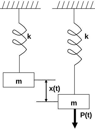
spring-mass system. The deflection shown in figure 4.1 has a time component dependent upon

the natural frequency of the span. Figure 4.4 depicts a simple spring model of a conductor span

where k is the spring constant, m is the system mass, P(t) is the applied force, and x(t) is the

displacement.

m k

m

P(t) x(t)

k

Figure 4.4: Spring-Mass System Representation of Rigid Bus Span

The dynamic analysis of the simple spring mass system is detailed in [9] and modeled by

the differential equation 4.2.

t) sin( P kx dt

x d

m _f

2 2

ω =

+ (4.2)

Because it has one degree of freedom, the X direction will be used to indicate motion of

the mass. On the rigid conductor spans depicted in figures 4.2 and 4.3, the direction of force is

with forced frequency, _f. In the case of a power system fault, the driving forces are the

electromagnetic forces described in section 3.2.

Solving equation 4.2 for displacement, x(t), results in equation 4.3 where P is the

amplitude of the driving force and _nis the system natural frequency.

2

n f 1

k P x(t)

  

 −

= (4.3)

The natural or circular system frequency is defined in equation 4.4. It is independent of

any outside forces and is the time required for steady state deflection to occur.

m k

n = (4.4)

The driving frequency should not be confused with the system natural frequency. The

system can be excited using any value of P(t) with distinct driving frequencies. In the case of the

span of rigid bus on the 60 Hz power grid as described in previous sections, these are primarily

120 Hz with a DC offset with some 60 Hz components dependent upon the system X/R ratio.

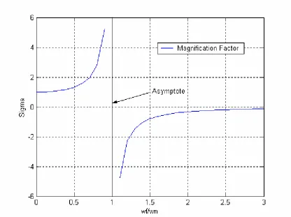
[10] discusses the concept of a magnification factor. The ratio of the displacement, x(t),

to the static displacement, -kx, is a magnification factor, (sigma), described in equation 4.5.

2

n f 1

1

k P x(t)

   

  − =

= (4.5)

Further analysis of equation 4.5 reveals an asymptote when the forced frequency is equal

Figure 4.5: Magnification Factor of a Spring-Mass System

The asymptote of figure 4.5 represents an interesting and common natural phenomenon.

Any system excited at its natural frequency appears to have infinite gain and maximum output

per given input. A simple example of this is a child in a swing. As the “pusher” of the swing, it

is often desirable to swing the child high with minimal effort. If the pusher adapts the frequency

of the pushes to match that of the rhythm of the swing, the mathematical representation is

depicted as the asymptote in figure 4.5. In reality, the swing would not have infinite gain to any

input due to wind resistance, imperfections in the hardware, and motion of the child. If the

swing is pushed at a rhythm not equal to the natural frequency, the “pusher” will have a difficult

time getting the swing to move higher (and would also have a disappointed child).

These same natural frequency characteristics apply to that of substation bus deflection. If

limits and create permanent damage. The major means of excitement for rigid bus are seismic,

wind, and electromagnetic. In general, it is desirable to design substation equipment such that

the natural frequencies of conductor spans do not have a chance of becoming excited with a large

magnification factor by any of these forces. For electromagnetic force excitement, the IEEE

recommends the use of dampers if the natural frequency of the conductor span is greater than the

power frequency [2]. Additionally, if twice the natural frequency of a span is greater than the

force driving frequency due to wind, damping is recommended. Damping commonly involves

the installation of flexible conductor inside a tubular conductor.

On the other hand, the natural frequency presents unique design characteristics. For

example, [11] presents the novel application of removal of ice from flexible bundled conductors

by exciting the span with frequencies near its fundamental frequency. This oscillatory

excitement causes conductor bundles to literally collide with each other and remove ice by these

collisions.

In the application of fault detection, the natural frequency of the bus span plays a key

role. In accordance with the magnification factor described in this section, the ratio of the

driving frequency to the rigid bus span’s natural frequency will be greater than unity. As in the

analogy of a child on a swing, the theoretical value of infinite gain cannot be reached by the

conductor driven at its natural frequency. This is mostly due to the resistance of the bus supports

and insulator supports and the damping it provides. Although this infinite gain characteristic

cannot be attained, it still represents the frequencies producing the most stress on the span.

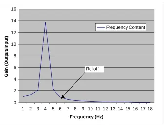
Figure 4.6 depicts a typical frequency response output for the spring mass system

depicted in figure 4.4. The peak gain is not infinite for the reasons described in this section. The

0 2 4 6 8 10 12 14 16

1 2 3 4 5 6 7 8 9 10 11 12 13 14 15 16 17 18

Fre que ncy (Hz)

G

ai

n (

O

ut

put

/I

nput

)

Frequency Content

Rolloff

Figure 4.6: Frequency Response of a Spring-Mass System

The components of rigid bus spans must be translated to parameters of the spring-mass

models for the purpose of dynamic analysis.

The natural frequency of a single bus span with fixed ends is defined in equation 4.6 as

described in [2].

m EI

L C

K f

2 2

n = (4.6)

where fn = natural frequency of conductor span

K = 1.51 for fixed ends on the conductor span

C = 24 for English units

L = conductor length (ft)

E = modulus of elasticity (lb/in2)

I = moment of inertia (in4)

The conductor spring constant, kbus, is determined by combining equations 4.4 and 4.6

into equation 4.7.

I E L C

K 4 k

4 2

4 4

bus = (4.7)

Figure 4.7 is an application of equation 4.6 to show several conductor’s natural frequency

versus length. The figure provides information that shows a correlation between the stiffness of

the conductor verses its natural frequency. Smaller natural frequencies correspond to larger and

stiffer conductors. Additionally, higher natural frequencies correspond to shorter conductor

spans These characteristics are useful in conductor selection in addition to ampacity/heat

requirements in [2].

5 10 15 20 25 30 35 40

0 10 20 30 40 50 60 70 80

Nat

ur

al

F

req

ue

nc

y

(Hz

)

Span Length (ft)

1" Schedule 40 Al Tubing 2-1/2" Schedule 40 Al Tubing 4" Schedule 40 Al Tubing 6" Schedule 40 Al Tubing 1/2" x 4" Al Flat Bar

The analogy of the spring-mass system should include the support insulators. Tips of the

insulators will move at their natural frequencies when driving forces are applied. [12] describes

the concept of a spring constant for insulator supports. This insulator spring constant is defined

in equation 4.8 where E is the section modulus, I is the moment of inertia, and H is the height of

the insulator.

H I E 3

k_ins = (4.8)

Equation 4.9 gives the natural frequency for insulators. In reality, this natural frequency

is the basis for determining tip displacement versus applied load to a span of conductor. Both the

natural frequencies for the bus span and insulator have been verified using the chirp response

method via adaptive filtering in [12].

b i ins ins

F F .226

g k 1

f

+

= (4.9)

where fins = insulator natural frequency

g = gravitational constant (386.4 in/s2)

Fi = insulator weight (lb)

Fb = effective weight of conductor transmitted to support fitting (lb)

The dynamic model for a single span of bus including the response of the insulators is

m₁ k_ins

m₁ x₁(t)

m₂ k_bus

m₂

P(t) x₂(t)

k_bus k_ins

Figure 4.8: Spring-Mass System Representation of Rigid Bus Span with Insulators

The dual spring-mass system of figure 4.8 can be electrically analyzed using the model in

figure 4.9.

L

=m

+

x

(t)

L

=m

C

=1/k

C

=1/k

P(t)

-+

-+

-R

Figure 4.9: Electrical Equivalent Model of a Mechanical Spring-Mass System

wind resistance would not dissipate any of the energy from the input source. This produces a

ringing effect which would never settle to any DC value.

The differential equations governing the electrical equivalent circuit are shown in

equations 4.10 and 4.11 (neglecting the resistance contribution). The mechanical system

equivalents are shown in equations 4.12 and 4.13.

0 C q q C q dt q d L 2 2 1 1 1 2 1 2 1 = − +

+ (4.10)

P(t) C q q dt q d L 2 1 2 2 2 2

2 + − = (4.11)

0 ) x (x k x k dt x d

m _{1 1 2 1 2}

2 1 2

1 + + − = (4.12)

P(t) ) x (x k dt x d

m _{2 2 1}

2 2 2

2 + − = (4.13)

The frequency response of the dual spring-mass system, figure 4.10, shows the presence

of two distinct natural frequencies. The smaller natural frequency is the conductor span’s

frequency and the larger is the insulator natural frequency. This is consistent with the

0 0.5 1 1.5 2 2.5

1 3 6 8 11 13 16 18 21 23

Frequency (Hz)

G

a

in

(O

ut

put

/I

n

put

) Frequency

Content

Natural Frequencies

Figure 4.10: Natural Frequencies of a Dual Spring-Mass System

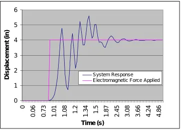
The transient step response for the system of figure 4.8 is depicted in figure 4.11. The

motion of the conductor is shown to have a swinging effect with damping contributions from

Rdamp. The period of oscillation for the response is the reciprocal of the fundamental (lowest and

most dominant natural) frequency of the conductor. The second natural frequency of the system

contributes its oscillating characteristics showing insulator tip displacement at the conductor

midspan. Since the driving frequencies are either 120 or 60 Hz, the motion of the spring-mass

system mostly moves due to DC components. This displacement is seen as the step response as

0 1 2 3 4 5 6 0 0. 06 0. 73 1. 01 1.

08 ₁.2

1.

34 ₁.5

1. 87 2. 45 3. 08 3. 66 4. 24 4. 86 Time (s) Di spl acem ent (i n) System Response

Electromagnetic Force Applied

Figure 4.11: Transient Step Response of a Dual Spring-Mass System

Determination of the system natural frequencies is accomplished using matrices for the

mechanical spring system in figure 4.8. The equations can be put into matrix form as written in

equations 4.14 and 4.15.

    =         − − + +                 0 0 x x k k k k k dt x d dt x d m 0 0 m 2 1 2 2 2 2 1 2 2 2 2 1 2 2 1 (4.14) 0 x K x

M&&+ = (4.15)

The matrix K is defined as the stiffness matrix for the system. Manipulation of the

differential equation matrices yields the determination of the natural frequencies for the system

[9] in equation 4.16.

0 ) I 2 -K 1 -M

where

M

K

I

= system natural frequencies (rad/s)

The eigenvalues of M-1K results in the determination the natural frequencies, 12and

22. The square root of the eigenvalues will result in the two natural frequencies of the system.

The mode shapes of the oscillatory spring-mass system are the eigenvectors of M-1K.

The system will have as many distinct mode shapes as the order of the matrices. Thus, the

system of the busbar with insulator supports contains two modes of oscillation. The actual free

motion of the system is determined using superposition of the various modal shapes of the linear

system. Because the first mode of oscillation is most dominant and the higher order modes are

less dominant, a system can be approximated using this superposition technique over the first

few modes.

By including the insulators in the model for displacement, a more accurate response can

be determined for the system than the busbar. To further improve the modeling, the natural

frequencies of the bus support structure should be included in the model. The IEEE indicates

further analysis is possible using the structure/insulator combination [2]. The use of single phase

lolly column support structures tends to absorb energy which reduces the displacement of the

bus. Because the analysis in this paper utilizes three phase bus supports with little self-deflection

due to canceling effects of faulted phases, the analysis of the influence of single phase bus

supports will not be covered. For the modeling in the application of figure 4.3, the effect of the

4.3 Dynamic Response of Bundled Conductor Faults

The displacement of bundled conductors during a fault should be equal and opposite as

depicted in figure 4.12 assuming minimal influence from outside phases. This is a characteristic

of the pinch effect discussed in section 3.

d(t) d(t)

i(t)

i(t)/2 i(t)/2

i(t)

L d

Figure 4.12: Bundled Conductor Displacement Due to Fault Forces

Equation 4.17 is an application of equation 3.4 with input current i(t)=isin(ωt)split

equally between both conductors.

d 2

t) ( sin (i/2) L F

2 2 o

ab

ω

= (4.17)

Figure 4.13 is a plot of equation 4.17 with magnitude of input current equal to 10 kA

0 0.005 0.01 0.015 0.02 0.025 0.03 0.035 0.04 0.045 0.05 0

0.1 0.2 0.3 0.4 0.5 0.6 0.7

Time (s)

F

or

c

e (#/

in)

Dynamic Force Average Force

Figure 4.13:Bundled Conductor Short Circuit Forces

The function is primarily driven by sin2(ωt). The sinusoidal function as an input signal

can be broken down into components and its outputs added together via superposition to attain

the system output. The sinusoidal half angle formula [13] can be applied to bundled conductors

to show the components of the linear system.

2 ) 2 cos( 2 1 2

t) cos(2 -1 t) ( 2

sin ω = ω = − wt (4.18)

Equation 4.18 indicates a DC component equal to half the peak time varying signal. The

AC component is equal to a sinusoidal component with frequency of twice the power frequency.

As discussed throughout section 4, system inputs with frequencies near the system

inputs to the system. The AC component in a 60 Hz electric system will show up as purely 120

Hz if the X/R ratio is considered negligible. The same holds true after the transient fault current

portions have subsided.

Figure 4.14 shows the influence from the transient portion of fault currents due to the

X/R ratios discussed in section 2. During the presence of the transient component, there is

significant influence from the 60 Hz and DC portions of fault current. The green and red arrows

indicate the development of a 120 Hz sinusoidal function, sin2(ωt), in the steady state. The 0,

60, and 120 Hz components are displayed in figure 3.7 via Fourier analysis.

The DC component in the steady state is present for the duration of the fault. The initial

DC component is also present, but varies according to the transient duration. Deflection of the

bus does not vary significantly with varying X/R ratios because the additional DC components

will decay faster than the bus can displace. The amount of DC component in the force signal is

0 0.02 0.04 0.06 0.08 0.1 0.12 0.14 0.16 0.18 0.2 0

0.5 1 1.5 2 2.5

Time (s)

Forc

e (#/

in)

Decaying Exponential Influence

Decaying Exponential Influence

Steady State Transient

Figure 4.14: Transient Bundled Conductor Short Circuit Forces

The deflection on a bus span to an input signal must be evaluated during design to ensure

the bus is not excited electrically near the natural frequencies of the bus span. Based on the

research of this paper and [2], it can be concluded that the higher order frequencies of the input

waveform have little influence on the bus span. The approach of using the DC component of the

fault current as the primary and most influential component of the conductor motion can be

utilized effectively, regardless of typical X/R ratios. For the purpose of this paper in its

recommendations for fault detection, the bus span’s natural frequencies should have negligible

have the most significant impact. The DC component input is the average of the electromagnetic

force generated. An example of this is depicted in figure 4.15.

0 0.02 0.04 0.06 0.08 0.1 0.12 0.14 0.16 0.18 0.2 0

0.5 1 1.5 2 2.5

Time (s)

For

c

e (

#

/in)

Dynamic Force Average Force

Figure 4.15: Average Bundled Conductor Short Circuit Forces

Using the average input force as the input function to the dual spring-mass system, the

displacement of the conductor midspan can be accurately modeled. The fundamental frequency

becomes the most important setting for the conductor response to this input function. It

primarily drives conductor deflection generally slower than the transient component of fault

current can influence deflection. This simplifies analysis of bundled conductor deflection by

5.0 Optical Method of Fault Detection

Electromechanical forces generated during power system faults affect all power system

equipment in series with the fault. This includes insulators, conductors, support structures,

breakers, transformers, and generators. Theoretically, any of these power system components

could be measured for the effects of fault current detection. For example, stresses on insulators

or structures could be measured using strain gauges. This paper focuses on the optical method of

detection in which the motion of the conductor span is measured at its midpoint. The span can

then be designed to provide accurate detection which can be integrated into a relay

time-overcurrent curve.

5.1 Physical Configuration

Conventional relay selection and settings require the use of set points to trigger action

upon detection of faults. The conductor dynamics approach to fault detection also requires set

points. The method for choosing a single set point will be discussed in this section. This set

point is the determined using the physical analysis of conductor deflection and integrating to the

electrical domain of relay settings.

Crucial to understanding the operation of the optical fault detection system is the

proposed physical configuration of figure 5.1. Each conductor is equipped with a reflective

mirror which reflects normal to the ground plane. Its purpose is to reflect a transmitted laser