Theoretical Derivation on the Fundamental Frequency of Variable thickness Conical Shells

2017 International Conference on Mathematics, Modelling and Simulation Technologies and Applications (MMSTA 2017) ISBN: 978-1-60595-530-8

Theoretical Derivation on the Fundamental Frequency of

Variable-thickness Conical Shells

Wei NING

*

_{, Feng-sheng PENG and Nan WANG}

School of Mechanical Engineering, Shaanxi University of Technology, Shaanxi, China *Corresponding author

Keywords: Conical shell, Generalized differential quadrature, Fundamental frequency.

Abstract. The fundamental frequencies of the variable thickness truncated conical shells with

different boundary conditions are studied by combining the vibration theory with the generalized differential quadrature method which is applied to discrete the derivatives in the governing equations. The discretization of the system leads to a standard linear eigenvalue problem. The coefficients of the governing equations are obtained by theoretical derivation and different boundary conditions are considered. The work can provide the theoretical evidences to design the conical shell for good structural performance.

Introduction

The truncated conical shell structures have increasingly been used in many fields such as space flight, rocketry, aviation and submarine technology, etc. Therefore, the frequency characteristics of the truncated hollow conical shell must be studied for safety and stability reasons. Maximization of the natural frequencies is good for vibration reduction, which is favorable for decreasing both of the steady state and transient response of the structure being excited. The available literature dealing with vibration of shells shows that great efforts have been devoted to this area, although much work is still needed to cover some other aspects. The majority of the existing literature describes the vibration analysis for thin conical shells and is based upon the Rayleigh-Ritz method and numerical integration method(Talebitooti et al.2010;Ye et al. 2014). Soedel (1993) studied the equations of motion for circular cylindrical and conical shells based on Rayleigh-Ritz principle. Siu and Bert(1970) have applied the Rayleigh-Ritz method to compute the frequencies for the free vibration of isotropic conical shells. Wang et al (1997) have also used the Ritz polynomial functions for axial modal dependence to analyze ring-stiffed cylindrical shells. These appeared to provide a good convergence to the Rayleigh-Ritz method. The work of Goldberg et al (1970) and Kalnins (1964) is aimed at the vibration analysis of isotropic conical shells by the numerical integration method. In some other works, Irie et al (1982,1984) studied the free vibration of conical shells to obtain the natural frequencies with variable thickness by using the matrix transfer method for a given set of boundary conditions. Cheung et al (1989) developed a spline finite strip method and studied the free vibration of singly curved shells. The power series expansion approach was used by Tong (1993a,1993b) to study the free vibration of orthotropic and composite laminated conical shells. The finite element method is widely used to obtain the computed eigenfrequencies of conical shells based on the numerical discretization of partial diffential equations (Sivadas et al.1991,1992;Dey et al,2014). The collocation method was implemented to solve the associated eigenvalue problem.

Governing Equations

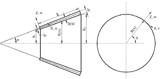
Figure 1. Geometry of the truncated conical shell with variable thickness.

Figure 1 shows the geometry of a variable thickness truncated circular conical shell with semi-vertex cone angle . The variation of the conical shell thickness, h x( ) is considered as a power

function expressed by the relation:

 

1 2 1

( ) , 0,1, 2

m

m

x h x h h h m

L      _{ } 

(1) where h1 and h2are the shell thickness at the small and large edges, respectively. L is the slant length

of the shell. Shells with uniform, linear or parabolic thickness distribution shall have values of integer exponent m equal to 0, 1 or 2, respectively. The equilibrium equation of motion in terms of the force and moment resultants can be written as

2

2

1 sin

( ) ( )

( ) ( )

x x

x t

N N u

N N x

x R x R x t



 

 

  

   

   ₍₂₎

2

2 2

1 2 sin cos cos

( )

( ) ( ) ( ) ( )

x x

x t

N N M M v

N x

x R x R x R x x R x t

   



  



 

    

    

     ₍₃₎

2 2 2 2

2 2 2 2

2 sin 2 sin 1

(sin cos ) ( )

( ) ( ) ( ) ( )

x x x

t

M M M M M w

N x

R x x R x x R x x

x R x t

  



 

  

 

     

     

   

   ₍₄₎

here t( )x is the density per unit length. Moment resultants and in-surface force can be obtained by

( ) ( )

( , , ) m ( , , )

m

h x

T T

x x x x

h x

M M_ M_   _{ } zdz





_

(5)

( ) ( )

( , , ) m ( , , )

m

h x

T T

x x _{h x} x x

N N N 



_     dz

(6) Based on the two-dimensional Hooke’s law, the stress vector is defined by( )T ( , , )

x  x

     and can be written as

11 12

12 22

66

x x

x x

Q Q Q Q

Q

 

 

 

 

 



    

    

    

  _{ } 

    ₍₇₎

where   T , ,  x  x

     is the strain vector. The stiffness Qijis defined as

11 2, 12 2, 22 2, 66

2(1 )

1 1 1

E E E E

Q Q  Q Q



  

   



[image:2.612.168.423.82.208.2]

where E and  are the Young’s modulus and Poisson’s ratio of the shell material. Based on the

Love’s first approximation theory, the strain components of this vector are defined as linear function of the normal coordinate z, namely

1 1

x z

    _, _ ₂z_2, x   2z (9)

where   1, ,2  and  1, 2, 2 are, respectively, the strain and curvature vectors of the reference

surface which are defined by

1

u x

 

 _{, (10)}

2

1 sin cos

( ) ( ) ( )

v u w

R x R x R x

 







  

 _{, (11)}

1 sin

( ) ( )

u v v R x x R x

 



 

  

  ₍₁₂₎

2

1 2

w x

  

 _{, (13)}

2

2 2 2 2

1 cos sin

( )

( ) ( )

w v w

R x x R x R x

 



 

  

   

 

 _{, (14)}

2

2 2

1 sin cos sin cos

( ) ( ) ( ) ( )

w w v v

R x x R x R x x R x

   



 

  

   

     ₍₁₅₎

By substituting Eqs (7)-(15) into Eqs (5)-(6), the force and moment resultants can be obtained as

1

11 12

12 22 2

66

( ) x

m

x

N Q Q

N h x Q Q Q N





  



    

    

   _{  } 

  _{   }

  _{, (16)}

1

11 12

3

12 22 2

66

( ) 12

2 x

m

x

M Q Q

h x

M Q Q

Q M





  



    

    

   _{  } 

  _{   }

  ₍₁₇₎

The displacement field can be expressed in shell coordinates



x, , z



as

( ) cos( ) cos( )

uU x  n  t ₍₁₈₎

( ) sin( ) cos( )

vV x  n  t ₍₁₉₎

( ) cos( ) cos( )

W x n t

     ₍₂₀₎

Substituting Eqs. (16)-(20) into Eqs. (2)-(4), the governing equations can be written as

2

2

110 111 112 2 120 121 130 131 t( )

U U V W

S U S S S V S S W S x U

x x x x  

   

       

    ₍₂₁₎

2 2

2

210 211 220 221 222 2 230 231 232 2 t( )

U V V W W

S U S S V S S S W S S x V

x x x x x  

    

        

2 2 3 4

2

310 311 320 321 322 2 330 331 332 2 333 3 334 4 t( )

U V V W W W W

S U S S V S S S W S S S S x W

x x x x x x x  

      

         

        ₍₂₃₎

The coefficientsSijkare given in the appendix.

In this study, the following two types of boundary conditions are considered. For a simply supported end (SS)

0

V  _,W 0_,Nx0,Mx0 (24) For a clamped end (C)

0

V  ,W 0,U0, 0 W

x 



 ₍₂₅₎

Generalized Differential Quadrature(GDQ)

The GDQ method developed byShu et al is numerical algorithm to approximate the solution of a partial differential equation based on the analysis of a high order polynomial approximation and the analysis of a linear vector space. For generality, GDQ chooses two sets of base polynomial to determine the weight coefficients. The weighting coefficients of the first order derivative are computed by a simple algebraic formulation while the weighting coefficients of the second and higher order are given by a recurrence relationship. For a smooth function f x t( , ), GDQ discretizes its

nth order derivative with respect to x at the grid point x_i, as

( ) ( )

1

( , ) ( , ), 1, 2, , 1, 1, 2, , N

n n

x i ik k

k

f x t c f x t n N i N







    

(26) where Nis the number of grid points in the x direction, x_iis the coordinate of the grid point, c( )ikn are

the weighting coefficients to be determined. For the first order weighting coefficients

1, (1)

1,

( )

, , 1, 2, , ,

( ) ( )

N

i k k k i

ij N

i j j k

k k j

x x

c i j N i j

x x x x

 

 



  

 







(27)

(1) (1)

1,

, 1, 2, , N

ii ij

j j i

c c i N

 

 



  (28)

For the second and higher order weighting coefficients

( 1)

( ) ( 1) (1) _{, , 1, 2, , ,}

n ij

n n

ij ii ij

i j

c

c n c c i j N i j x x

 

   



 

 

 

   (29)

( ) ( )

1,

, 1, 2, , N

n n

ii ij

j j i

c c i N

 

 



  (30)

In the following, the fundamental eigenfrequency of the isotropic variable-thickness conical shell is studied under four sets of boundary conditions, namely, the simply supported small and large ends (SS-SS); the simply supported small end and clamped large end (SS-C); the clamped small end and simply supported large end (C-SS); and the clamped small and large ends(C-C). The GDQ method is applied to discretize the derivatives in the governing equations and the boundary conditions. For the spatial discretization, the coordinates of grid points are chosen as

0.5 {1 cos[( 1) / ( 1)]}, 1, 2, ,

The governing equations (21-23) can be spatially discretized by using the GDQ method and becomes

(1) (2) (1) (1) 2

110 111 112 120 121 130 131

1 1 1

( )

( ) t

N N N

i ik ik k i ik k i ik k i

k k k

x

S U S c S c U S V S c V S W S c W  U

  





  



 



 

(32)

(1) (1) ( 2) (1) ( 2) 2

210 211 220 221 222 230 231 232

1 1 1

( ) ( ) ( )

N N N

i ik k i ik ik k i ik ik k t i

k k k

S U S c U S V S c S c V S W S c S c W  xV

  





 



  



   (33)

(1) (1) (2)

310 311 320 321 322 330

1 1

(1) (2) (3) (4) 2

331 332 333 334

1

( )

( ) ( )

N N

i ik k i ik ik k i

k k

N

ik ik ik ik k t i

k

S U S c U S V S c S c V S W

S c S c S c S c W  xW

 



    

    







(34)

After spatial discretization, for simplicity, the boundary condition of the simply supported small end and clamped large end (SS-C) is considered and the boundary condition (SS) at the small end can be written as

1 0

V  ,W10 (35)





1

(1) (1)

11 1 1

2

N

Q k k

k

c C U c U





  



(36)







   







2

(2) (1) (2) (1) (2) (1)

12 12 2 1 1 1 1 1 1 1

3

N

Q N Q N N k Q k k

k

c C c W c C c W c C c W



  



    



 (37)

where 12 11 1 sin Q Q C Q R 

 (38)

The boundary condition (C) discretized by GDQ at the large end can be written as

0 N

V  ,W_N 0,U_N 0, (39)

 

2

(1) (1) (1)

2 2 1 1

3

N

N N N N Nk k

k

c W c W c W

  



  



(40)

The boundary condition equations can be coupled to provide the solutions U1, W2, W_N₁ as

1 (1) 1 2 1 (1) 12 11 11 1 sin N k k k c U U Q c Q R      



(41) (1) (1) 2

12 1( 1)

(1) (2) 12 1 (1) (2)

( 1) 1 1( 1)

3 11 1 11 1

2 (1) (1)

12 1( 1)

(1) (2) (1) (2) 12 12

2 1( 1) ( 1) 12

11 1 11 1

sin sin sin sin N N k

N N k Nk N k

k

N

N N N N

Q c

Q c

c c c c W

Q R Q R

W

Q c Q c

c c c c

Q R Q R

                       _{ }                   _{ }  



(42) (1) (1) 2 12 12)

(1) (2) 12 1 (1) (2)

2 1 12

3 11 1 11 1

1 (1) (1)

12 1( 1)

(1) (2) (1) (2) 12 12

2 1( 1) ( 1) 12

11 1 11 1

sin sin

sin sin

N

k

N k Nk k

k N

N

N N N N

Q c

Q c

c c c c W

Q R Q R

W

Q c Q c

c c c c

Q R Q R

By substituting boundary condition equations into governing equations, the eigenvalue equation system can be obtained

 

A

 

X  

 

X (44) where

  

2, , 1, , ,2 1, 3, , 2



T

N N N

X  U U _ V V _ W W _ ,  2 .Solving the eigenvalue of matrix

 

A provides the nature frequencies of the conical shells.

Conclusions

In this paper, an analysis is presented for the free vibration of truncated conical shells with variable thickness. Four sets of boundary conditions, namely, the simply supported small and large ends (SS-SS); the simply supported small end and clamped large end (SS-C); the clamped small end and simply supported large end (C-SS) and the clamped small and large ends(C-C) are considered. In the presented study, the thickness modes of the truncated shells include uniform thickness distribution, linear thickness distribution and parabolic thickness distribution. The shell governing equations are established using Love’s first approximation thin shell theory. The generalized differential quadrature method is applied to discretize the derivatives in the governing equations and different boundary conditions.

Acknowledgments

The authors are grateful for the financial support by Science and Technology Project of Shaanxi University(No. SLGQD14-03), Shaanxi Provincial Department of Education Research Fund funded projects(No.15JK1133),Natural Science Project of Shaanxi Provincial Science and Technology Department(No. 2016JM5039) and National Science Youth Fund(No. 51605269).

References

[1] Ye. T., Jin. G., Su. Z., Jia. X. “A unified Chebyshev–Ritz formulation for vibration analysis of composite laminated deep open shells with arbitrary boundary conditions”. Arch. Appl. Mech. 2014(84) ,p. 441-471.

[2] Soedal W. “Vibration of Shells and Plates, 2nd ed. Marcel Dekker, New York, 1993.

Siu C.C, Bert C.W. “Free vibration analysis of sandwich conical shells with free edges”. J. Acoust. Soc. Am. 1970(47), p. 943-945.

[3] Wang C.M, Swaddiwudhipong. S., Tian J., “Ritz Method for Vibration Analysis of Cylindrical Shells with Ring Stiffeners”. J. Eng. Mech. 1997(123), p. 134-142.

[4] Goldberg J.E, Bogdanoff J.L., Marcus L. “On the calculation of the axisymmetric modes and frequencies of conical shells”, J. Acoust. Soc. Am. 1970 (32), p. 738-742.

[5] Kalnins A. “Free Vibration of Rotationally Symmetric Shells”. J. Acoust. Soc. Am1964 (36), p. 1335-1365.

[6] Irie T., Yamada. G., Kaneko Y. “Free Vibration of a Conical Shell with Variable Thickness”, J. Sound. Vib. 1982(82), p. 83-94.

[7] Irie T., Yamada G., Kaneko Y.: “Natural Frequencies of Truncated Conical Shells”. J. Sound. Vib. 1984 (92), p. 447-453.

[8] Cheung Y.K, Li. W.Y, Tham L.G.“ Free Vibration Analysis of singly Curved Shell by Spline Finite Strip Method”. J. Sound. Vib. 1989 (128), p. 411-422.

[10]Tong L.Y. “Free Vibration of Composite Laminated Conical Shells”. Int. J. Mech. Sci. 1993 (35), p. 47-61.

[11] Sivadas. K.R., Ganesan. N.: “Vibration analysis of laminated conical shells with variable thickness”. J. Sound. Vib. 1991 (148), p477-491

[12] Sivadas. K.R, Ganesan. N. “Vibration analysis of thick composite clamped conical shells of varying thickness”. J. Sound. Vib. 1992 (152), p27-37.