A New Feedback Linearization-NSGA-II based Control
Design for PEM Fuel Cell
Alireza Abaspour
Space Research Institute Maleke_ashtar University of
Technology Tehran, Iran
Nasrin Tadrisi Parsa
Department of Electrical Engineering, Islamic Azad University,
Damavand, Iran
Mohammad Sadeghi
Space Research Institute Maleke_ashtar University of
Technology Tehran, Iran
ABSTRACT
This paper presents a new method to design nonlinear feedback linearization controller for polymer electrolyte membrane fuel cells (PEMFCs). A nonlinear controller is designed based on nonlinear model to prolong the stack life of PEM fuel cells. Since it is known that large deviations between hydrogen and oxygen partial pressures can cause severe membrane damage in the fuel cell, feedback linearization is applied to the PEM fuel cell system, thus the deviation can be kept as small as possible during disturbances or load variations. To obtain an accurate feedback linearization controller, tuning the linear parameters are always important. So in proposed study NSGA_II method was used to tune the designed controller in aim to decrease the controller tracking error. The simulation result showed that the proposed method tuned the controller efficiently.
General Terms
PEM Fuel Cell, Nonlinear Control, Optimization .
Keywords
Nonlinear dynamic model, Polymer electrolyte membrane Fuel cells, Feedback linearization, Optimal control, NSGA_II.
1.
INTRODUCTION
A FUEL cell is an electrochemical energy device that by using chemical reaction converts the chemical energy of fuel directly into electricity. The product of this chemical reaction are heat and water which make it as one of the most environmentally friendly energy. The high energy efficiency, extremely low emission of oxides of nitrogen and sulfur, and very low noise, as well as the cleanness of its energy production lead to consider this renewable energy source as one of the most favorable energy.
To generate an efficient and trustworthy power response and to prevent membrane damage such as detrimental degradation of the stack voltage and oxygen depletion, it is necessary to design a better control scheme to achieve optimal air and hydrogen inlet flow rates.
To design an efficient nonlinear control scheme, it is necessary to obtain a PEMFC accurate mathematical modeled. Several researches has been done, for obtaining the PEMFC model, ranging from stationary and dynamic models [1],[2],[3],[4], [5], [6] to the control design applied to a fuel cell vehicle and a distributed generation system [7], [8].
In order to use advanced controller techniques, it is essential to obtain an accurate nonlinear dynamic model of fuel cell
system which considers the system nonlinearities and uncertainties.
A control-oriented PEMFC model developed by Purkrushpan et al.[1]. This model includes flow characteristics and dynamics of the compressor and the manifold (anode and cathode), reactant partial pressures, and membrane humidity. The nonlinear relationship between stack voltage and load, and the state equations [1], [5], made the nonlinear control development of the PEMFC as a challenge for the control designers.
In Ref.[9] a fuzzy control system is designed for a boost dc/dc converter of a fuel cell system [9]. Ref.[10] presents a an optimal control design for the PEMFC using artificial neural network (ANN). In this design instead of controlling the PEM fuel cell system, the neural optimal control is mainly used to find a new architecture to develop an approximated optimal control by means of the ANN, where the PEM fuel cell was chosen as a test bed. Ref.[11] introduced a comprehensive nonlinear model which is utilizable for feedback linearization control. An adaptive inverse controller using radial basis function neural network (RBFNN) to PEMFC system is designed in [12]. This control scheme has the advantage of not needing to identify the dynamical parameters of the system for design and scheduling of the controller parameters. Also an adaptive controller for PEM is designed on [13], the adaptive 2DOF controller is used in order to obtain certain control performances for membrane conductivity management. The controller is implemented with 2 PID structures and an adaptation rule which was based on gain-scheduling method.
In this paper a nonlinear model of PEMFC based on [11] is used, then feedback linearization controller is designed to control the hydrogen and oxygen partial pressure. For improving the accuracy of proposed design, the linear control parameter of designed controller should be tuned. It is common to use pole placement or Lyapunov theory to obtain linear control parameter, but it is not an accurate way to tune these parameters. So the NSGA_II is used as an optimization algorithm to tune these parameter. Based on [14], NSGA-II, in most problems, is able to find much better spread of solutions and better convergence near the true optimal solution compared to other Evolutionary Algorithm (EA). Based on author research there is no report of using this method for optimizing the feedback linearization parameters. The simulation result showed that by using this method more accurate and precise feedback linearization is achieved.
proceed, whereas feedback linearization method explained in section 3, and the procedure to design stabilizing controller is illustrated on section 4. The NSGA-II explained in section 5. Then in section 6 the numerical simulation of classic feedback linearization, linear control and introduced method is done, while the conclusions are provided in section 7.
2.
DYNAMIC MODEL OF PEMFC
A PEM fuel cell consists of a polymer electrolyte membrane which is sandwiched between two electrodes (anode and cathode). In the electrolyte, only ions can exit and electrons are not allowed to pass through. Therefore, the flow of electrons needs a tool such as an external circuit between anode and cathode to produce electricity which caused by potential difference between them.
The overall electrochemical reactions for the PEM fuel happens between hydrogen-containing anode gas and an oxygen-containing cathode gas which produce water, heat and electricity is described as follows:
2
2 2
2 2 2
2
4
4
:
4
4
2
:
2
:
2
H
H
e
Cathode O
H
e
H O
Overall
H
O
H O electricity
hea
Anode
t
The PEMFC is composed of the following components as shown in Fig. 1: Anode Plate, Anode Gas Diffusion Layer, Anode Catalyst Layer, Proton Exchange Membrane, Cathode Catalyst Layer, Cathode Gas Diffusion Layer and Cathode Plate. From Anode side, the hydrogen enters through the anode gas diffusion layer (GDL) and reaches the anode catalyst layer (CL). Here, in the presence of the catalyst, hydrogen separates from its electron and travels through the proton exchange membrane on the other side as proton H. Meanwhile, the electron is transferred through the load towards the cathode plate where it reaches the cathode GDL.
Oxygen molecules, O2, which are present in the cathode GDL, in presence of catalyst on cathode side, will be separated into individual oxygen atoms and further a combination reaction takes place. One oxygen atom and two
H
protons with a couple of electrons coming through the load, they form an H2O water molecule. During this reaction, an electromotive force is exhibited with respect to the load and heat is released in the environment. [image:2.595.325.520.79.283.2]On the anode side, a fuel processor, which is called reformer, generates hydrogen through reforming methane or other fuels like natural gas, can be used instead of the pressurized hydrogen tank. A pressure regulator and purging of the hydrogen component are also needed. On the cathode side, an air supply system containing a compressor, an air filter, and an air flow controller are required to maintain the oxygen partial pressure. On both sides, a humidifier is needed to prevent dehydration of fuel cell membrane. In addition, a heat exchanger, a water tank, a water separator, and a pump may be needed for water and heat management in the FC systems [15], [16], [17].
Figure 1. Proton Exchange Membrane Fuel Cell schematic representation
Based on the polarization I–V curve, which expresses the relationship between stack voltage and load current [15], [17], a single cell produces voltage between 0 and 1 V , so to produce a higher voltage, multiple cells have to be connected in series. Fig. 2 shows the I-V curve nonlinear relationship which is mainly depends on current density, cell temperature, reactant partial pressure, and membrane humidity.
Figure 2. Polarization curve at 70C [15]
The output stack voltage
V
st [15] is defined as a function of the stack current, reactant partial pressures, fuel cell temperature, and membrane humidity:st activation ohmic concentration
V
E V
V
V
(1)In above equation, E is the thermodynamic potential of the cell or reversible voltage based on the Nernst equation,
activation
V is the voltage loss due to the rate of reactions on the surface of the electrodes, Vohmicis the ohmic voltage drop from the resistances of proton flow in the electrolyte, and
concetration
[image:2.595.317.531.402.510.2]Their equations are given as follows [15]:
2 2 2
0
[
0(
/ 2 ) ln(
H O/
H c)]
E
N V
RT
F
P
P
P O
(2)ln
2
fc n activation oI
I
RT
V
N
F
I
(3) ohm fcV NI r (4)
exp( )
concentration fc
V Nm nI (5)
Where 2 H
P
, 2 OP
, and2 C
H O
P
are the partial pressures ofhydrogen, oxygen, and water, respectively. Subscript c means the water partial pressure, which is vented from the cathode side. See Table.1 for cell voltage parameters.
Table1. Cell voltage parameters Definition
Parameter
Cell Number N
Open Cell voltage [V] 0
V
Universal gas constant [ j gm mol/ k] R
Temperature of the fuel cell [K] T
Faraday constant F
Charge transfer coefficient
Output current density[ 2 / A cm ]
fc
I
Exchange current density [ 2 / A cm ] 0
I
Internal current density [A cm/ 2]
n
I
Constant in the mass transfer voltage and
m n
Area-specific resistance [k cm 2] r
The nonlinear equation of PEMFC Anode and Cathode side are obtained from[11] as follows:
Anode side Equations :
2
2 2 1 ( 2 1 ) 2
H
a a H H fc a a H fc H
A
dP RT
u k Y C I u k C I F
dt V
(6)
2 2
2 2
2 2 2 2
a
A
A
a vs
a a H
H O
H H O a vs
A
a a H fc H O fc
P u k
dP RT P P P
dt V
u k C I F C I
(7)
Cathode side Equations:
2
2 2 2
1 1
2 2
O
c c O air fc c c N air fc O
C
dP RT C C
u k Y I u k Y I F
dt V
(8) 2 2 2 N
c c N air c c air N
C
dP
RT
u k Y
u k
F
dt
V
(9)
2
2 2 2
2
1
1 2 2
( )
C
c
c
c vs
c c air fc
H O
O N H O c vs
C
c c air fc fc H O fc
P
u k C I
dP RT
P P P P
dt V
u k C I C I F C I
(10)where uaand ucare the input control variables, ka and c
k the conversion factors,
2, 2, 2
H O N
Y Y Y are the initial mole fractions and set to be 0.99, 0.21, and 0.79, respectively. a andc are the relative humidity's on the anode and the cathode sides, respectively, Pvs is the saturation pressure, which can be found in the thermodynamics tables,
2
H
F ,F OH2 A,FO2,FN2and FH O2c are the pressure fractions of
gases inside the fuel cell, given as follows:
2 2
2 2 2 2 2
2 2
2 2
2 2 2 2 2
2 2
2 2 2
2
2 ,
, c A A A c A C C C H O O H
O N H O H H O
N H O
N H O
O N H O H H O
H O H O
O N H O
P P
F F
P P P P P
P P
F F
P P P P P
P F
P P P
(11)
3.
FEEDBACK LINEARIZATION
CONTROL
In this section, the feedback linearization technique is presented. Feedback linearization is a control design methodology that uses a feedback signal to cancel inherent dynamics and simultaneously achieves a specified desired dynamic response [18].
To exemplify the working principle of the feedback linearization, consider a system of order n with the same number m of inputs u and outputs y and affine in the control inputs. This type of system can be mathematically represented by:
( ) ( )
( )
x f x G x u y h x
(12)
where f and hare vector fields in n
R and m
R , respectively, and G is a
n m
control effectiveness matrix. The procedure to obtain the feedback linearization for system inversion consists of consecutive time differentiations of y until an explicit dependence on u appears. To each derivative, a new state vector is associated and the derivative of the last state vector is given by a nonlinear expression (the virtual control) to complete the transformation[19].Assuming now h x( )x, the first-order time-derivative of y is given by:
( )
( )
y
x
f x
G x u
(13)Since an explicit dependence on
u
was already found, the linear relation can be imposed (ifG x( )0 ) by selecting:1
( ) [
( )]
u
G x
x
f x
(14)1
( ) [
d( )]
u
G x
x
f x
(15)Where subscript d denote the desired dynamic. The desired dynamic is usually obtained by linear controllers, such as PD, PI or PID.
3.1
Controller Design
Up to here the MIMO dynamic nonlinear model of PEMFC is derived from (6-10), and the structure of feedback linearization controller is illustrated. In this section the procedure of implementing feedback linearization controller on a PEM fuel cell is stated. Feedback linearization is used in order to minimize the difference ∆P between the hydrogen and oxygen partial pressures. The main purpose of keeping ∆P in a certain small range is to protect the membrane from damage, and therefore, prolong the fuel cell stack life [1], [20].
Because the fuel cell voltage is a function of the pressures, each pressure needs to be appropriately controlled to avoid a detrimental degradation of the fuel cell voltage. The stack current is considered as a disturbance to the system instead of an external input [21].
Consider the following MIMO nonlinear system with a disturbance: 1 1 1
1, 2,...
( )
( )
( ) ,
( )
( )
,
m i i i m mi
m
X
f X
g X u
p X d
y
h X
y
h x
(16)Where n
XR is the state vector, m
UR is the input or control vector, P
yR is the output vector, f x
and g x
,1, 2,...,
i m ,are n-dimensional smooth vector fields. The d represents the disturbance variables, andp x
is the dimensional vector field directly related to the disturbance.By considering (6-10), the defined outputs and the disturbance, and separating the control inputs, the nonlinear dynamic system model of PEMFC is rewritten as follows:
1 1 2 2
1 1 1 3 2 2
( )
( )
( )
( )
( )
( )
X
f x
g x u
g x u
p x d
x
y
h x
x
y
h x
(17) Where: 2 2 2 2 2 2 2;
;
; ( )
0;
A C H H O O N H H a c t O O fcP
u
P
P
P
X
P
P
U
Y
u
P
d
I
f x
2 2 1 1 2 11 2 1 2
1( ) ( )
0 0 0
a H a
A A
a a vs a
A a vs A
H
k Y k x
V V x x
k P k x
V x x P V x x
g x RT
2 2 3
3 4 5
2
4
3 4 5
5
3 4 5 3 4 5
0 0
( )
( )
c O c
C C
air
c N c
C C
c c vs c
C c vs c
k Y k x
V V x x x
g x RT
k Y k x
V V x x x
k P k x
V x x x P V x x x
1 1 1
1 2
1 2 1
1 2
1 1 2
3 4 5
1 5 2 5
1 2
3 4 5 3 4 5
( )
( )
( )
2 2 ( )
0
( ) ( )
A A
A A
c C
C c C C
C C x
V V x x
C x C
V x x V
p x RT C C x
V V x x x
C x C x
C C
V V x x x V x x x V
From (17), the MIMO nonlinear PEMFC system is ready to develop a nonlinear control law. Normally, the disturbance in (17) cannot be directly used in the control design because an additional necessary condition—that the disturbance can be measured and the feed-forward action is allowed—has to be satisfied [22], [23].
Otherwise, the linearized map between the new input v and the output
y
does not exist. The condition renders the following control law by using the measurement of the disturbance:1( ) ( ) 1( ) 1( ) ( )
U A x f x A x vA x p x d (18) From (17), it can be seen that
f x
0
, that leads to:1 1
( ) ( ) ( )
UA x vA x p x d (19) Because each control variable u shows up after the first derivative of each
y
1
x
1 ,y
2
x
3, the relative degree vector
r
1r
2
is
1 1
, and the decoupling matrixA x
is defined as: 1 2 1 2 1 1 2 2( )
( )
( )
( )
( )
g g g gL h x
L h x
A x
L h x
L h x
(20) Where1 1
( )
g
2 2 2
2 1 1 2
3 3 4 5
0 ( )
0
a H H a H
A A
c O air c air
C c
k Y k Y x
V V x x
A x
k Y k x
V V x x x
(21)
( )
A x is nonsingular at
x
x
0. Additionally, the matrix v andp x
in (19) are given as follows:1 1 1
1 2
1 1
1 2
3 4 5
.
( )
( )
2 2 ( )
A A
C C
C C x
V V x x p x RT
C C
V V x x
y y
x v
(22)
The control law given in (18) yields decoupled and linearized
input–output behavior :
2
2
1 2
H
O
P
v
P
v
(23)
The outputs PH2and PO2are decoupled in terms of the new inputs v1 andv2. Thus, two linear subsystems, which are between the input
v
1 and the hydrogen partial pressure2
1 H
y P , and between the input
v
2 and the oxygen partial pressure y2PO2, are obtained. By mentioning that1 1
y
x
andy
2
x
3, in order to ensure thaty
1 andy
2 are adjusted to the desired values (in atmosphere) ofy
1d and2d
y
, the stabilizing controller is usually designed by linear control theory using the pole-placement strategy [24].In this paper NSGA_II method is introduced to design the stabilizer controller and the result will be compared with designed controller in [11].
4.
STABILIZING CONTROLLER
The outputs 2 H
P and 2 O
P are decoupled in terms of the new
inputsv1 andv2. Thus, two linear subsystems, which are between the inputv1and the hydrogen partial pressurey1PH2,
and between the input
v
2 and the oxygen partial pressure 22 O
y P , are obtained. Furthermore, note that y1x1 and
2 3
y x, so in order to ensure that y1 andy2 are adjusted to the desired values 3 (in atmosphere) of
y
1dandy
2d,the stabilizing controller is designed by linear control theory using the pole-placement strategy [24]. The new control inputs are given by1 11 1 1
2 21 2 2
d
d
y
k e
v
y
k e
v
(24)
Where
e
1
y
1y
1d,e
2
y
2
y
2d.Even though the nonlinear system PEMFC is exactly linearized by feedback linearization, there may exist a tracking error in the variation of the parameters, especially when the load changes. To eliminate this tracking error, the integral terms are added in the closed-loop error equation as in [23] and [11]:
1 11 1 12 1 1
2 2 21 2 22 2
d
d
y
k e
k
e dt
v
v
y
k e
k
e dt
(25)
From (24), the error dynamics can be obtained as follows:
1 11 1 12 21 2 22 2
0
0
e
k e
k e
e
k e
k e
(26)
By appropriately choosing the roots of the characteristics
of s2k s11 k12 and s2k s21 k22, asymptotic tracking will be achieved.
The overshoots also become small by choosing 2
11 412
k k and k2214k22 [23], [24].
[image:5.595.76.520.588.754.2]5.
NSGA_II
Technique that is widely applied in optimization problems. This is especially useful for complex optimization problems where the number of parameters is large and the analytical solutions are difficult to obtain. As it mentioned before, tuning the linear controller gain is really crucial for obtaining an accurate controller, therefore in this paper, a non-dominated sorting-based multi-objective EA (MOEA), called non-dominated sorting genetic algorithm II (NSGA-II) is suggested. This method is selected to alleviate these problem of other MOEA methods: 1) Computational complexity, 2) Non-elitism approach, 3) The need for specifying a sharing parameter [14]. By using this method, it is tried to optimize the PI linear parameter which have significant role in the behavior of designed controller. In optimization process the following objectives are considered:
1) Minimizing the 2 H
P tracking error.
2) Minimizing the 2 O
P tracking error.
In standard NSGA-II Crossover probability Pc is 0.9 and
mutation probability Pmis
1
n, wherenis the number of
decision variables, in which in this papernis 12 .The distribution indices for crossover and mutation operators are
20
c
and m20respectively.
In the optimization process, the population size is 20, and optimization repeated for 100 generation. The range of decision variable for controller gain is selected between 0.1 and 100. These variable range selection is based on numerous simulation result, to eliminate the singularity in simulations.
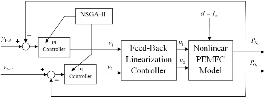
6.
NUMERICAL SIMULATION
In this paper a new combination of feedback linearization control and NSGA_II is used as it described. The overall view of designed controller is depicted on Fig.3. The NSGA-II algorithm is used to choose the optimal parameter of PI controller. To find the effectiveness of the introduced method the result of this new method should be compared with classical methods such as linear PI controller and also pure feedback linearization. In feedback linearization control, it is common to use pole-placement method to choose the linear controller gains, so the introduced method is compared with this procedure. The reference model parameters in (26) were selected as
k
12
k
22
5
andk
11
k
21
1
to establish the mentioned condition.While in this paper these gains is selected by NSGA-II method, to obtain accurate gains, which have significant effect on controller accuracy [25].
[image:6.595.318.522.74.204.2]As it can be seen on Fig.3, two PI controller gain should be tuned. Therefore 4 parameters are tuned by the NSGA-II optimization algorithm The result of optimization process is shown on Fig.4.
Figure 4. The final result of NSGA-II optimization process
As it can be seen on Fig.3 a single optimized point is obtained. By selecting this point the controller gains quantized as following:
1 11
22 2
12
153.149735,
21.646415
97.808318
,
12.511219
k
k
k
k
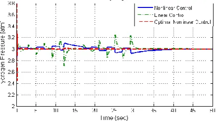
[image:6.595.321.541.371.493.2]The results of numerical simulation are presented on Fig.5, 6, 7,8,9,10. As it can be seen on Fig.5 and Fig.6 , by using the PD_NSGA method, a much more accurate controller is obtained, and the desired value (3 atmosphere) is obtained in proposed design, while the linear and nonlinear controller were incapable in accurate pressure control of desired values..
Figure 5.The comparison of Hydrogen pressure control
Figure 6. The comparison of Oxygen pressure control
[image:6.595.321.540.489.647.2]Figure 7.Variation of Hydrogen flow rate
Figure 8.Variation of Oxygen flow rate
Figure 9. Comparison of control effort
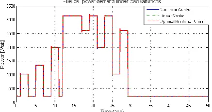
At the end as it can be seen in Fig.10, the power demand on the given load variation is supplied in all of the introduced controller, which confirms that beside the mentioned benefit of this new approach, the power supply of the controller remained constant.
Figure 10. Fuel cell power demand under load variation
7.
CONCLUSION
In this paper a new approach for designing optimal feedback linearization controller for PEM fuel cell is introduced. The accuracy of feedback linearization method depends on linear controller gains which are attached to it. These linear gains are usually obtained by classical methods, such as pole placement. These method suffer from lack of accuracy. So in this paper to tackle this problem, NSGA-II is introduced for tuning the linear control parameters. By using this method, the linear control parameters are tuned by considering the desired objectives in an optimal way. The simulation results, shows that the proposed method significantly increased the feedback linearization controller accuracy. Also this new designed controller achieved absolute minimum control effort which leads to saving energy instead of use the energy for control purposes.
8.
REFERENCES
[1] J. Purkrushpan, A. G. Stefanopoulou, and H. Peng, “Control of fuel cell breathing,” IEEE Control Syst. Mag., vol. 24, no. 2, pp. 30–46, Apr. 2004.
[2] M. J. Khan and M. T. Labal, “Dynamic modeling and simulation of a fuel cell generator,” Fuel Cells, vol. 5, no. 1, pp. 97–104, 2005.
[3] P. Famouri and R. S. Gemmen, “Electrochemical circuit model of a PEM fuel cell” in Proc. IEEE Power Eng. Soc. Gen. Meet., Jul. 2003, vol. 3, pp. 13–17.
[4] C. Wang, M. H. Nehrir, and S. R. Shaw, “Dynamic model and model validation for PEM fuel cells using electrical circuits,” IEEE Trans. Energy Convers., vol. 20, no. 2, pp. 442–451, Jun. 2005.
[5] L. Y. Chiu, B. Diong, and R. S. Gemmen, “An improve small-signal mode of the dynamic behavior of PEM fuel cells,” IEEE Trans. Ind. Appl ., vol. 40, no. 4, pp. 970– 977, Jul./Aug. 2004.
[6] J. M. Correa, F. A. Farret, and L. N. Canha, “An analysis of the dynamic performance of proton exchange membrane fuel cells using an electrochemical model,” in Proc. 27th Annu. Conf. IEEE Ind. Electron. Soc. IECON 2001, vol. 1, pp. 141–146.
[7] C. J. Hatiziadoniu, A. A. Lobo, F Pourboghrat, and M. Daneshdoot, “A simplified dynamic model of grid connected fuel-cell generators” IEEE Trans. Power Del., vol. 17, no. 2, pp. 467–473, Apr. 2002.
[image:7.595.54.280.277.531.2]power plant” IEEE Trans. Power Del., vol. 19, no. 4, pp. 2022–2028, Nov. 2004.
[9] A Sakhare, A Davari, and A Feliachi, “Fuzzy logic control of fuel cell for stand-alone and grid connection” J. Power Sources, vol. 135, no. 1/2, pp. 165–176, Sep. 2004.
[10] P. E. M. Almeida and M. Godoy, “Neural optimal control of PEM fuel cells with parametric CMAC network” IEEE Trans. Ind. Appl., vol. 41, no. 1, pp. 237–245, Jan./Feb. 2005.
[11] Woon ki Na and Bei Gou, "Feedback Linearization Based Nonlinear Control for PEM Fuel Cells" IEEE Transaction on Energy Conversion, 2008, Volume 23, Issue 1, March 2008 Page(s):179 – 190.
[12] A. Rezazadeh, A. Askarzadeh, M. Sedighizadeh "Adaptive Inverse Control of Proton Exchange Membrane Fuel Cell Using RBF Neural Network" International Journal of electrochemical science, Volume 6, pp.3105 - 3117, 2011.
[13] Alin C. Fărcaş, Petru Dobra "Adaptive control of membrane conductivity of PEM fuel cell" Journal of Procedia Technology , Vo.12, pp:42 – 49, 2014.
[14] Kalyanmoy Deb, Amrit Pratap, Sameer Agarwal, and T. Meyarivan "A Fast and Elitist Multi objective Genetic Algorithm:NSGA-II.",IEEE transactions on evolutionary computation, vol. 6, no. 2, april 2002.
[15] J. Larminie and A. Dicks, Fuel Cell Systems Explained.NewYork:Wiley, 2002
[16] J. Purkrushpan and H. Peng, "Control of Fuel Cell Power Systems: Principle, Modeling, Analysis and Feedback Design". Berlin, Germany: Springer-Verlag, 2004.
[17] F. Barbir, "PEM Fuel Cells: Theory and Practice". London, U.K. Elsevier, 2005.
[18] Reiner, J., Balas, G. J., and Garrard, W . L., “Robust Dynamic Inversion for Control of Highly Maneuverable Aircraft” Journal of Guidance, Control and Dynamics, V ol. 18, No. 1, 1995, pp. 18–24.
[19] Enns, D., Bugajski, D., Hendrick, D., & Stein, G. 1994. "Dynamic inversion: An evolving methodology for flight control design." International Journal of Control, 59,71– 90.
[20] W. Yang, B. Bates, N. Fletcher, and R. Pow, “Control challenges and methodologies in fuel cell vehicle development,” presented at the SAE, Paper 98C054, 1998.
[21] L. Y. Chiu, B. Diong, and R. S. Gemmen, “An improve small-signal mode of the dynamic behavior of PEM fuel cells,” IEEE Trans. Ind. Appl ., vol. 40, no. 4, pp. 970– 977, Jul./Aug. 2004.
[22] A. Isidori,"Nonlinear Control Systems", 3rd ed. London, U.K.: SpringerVerlag, 1995.
[23] M. A. Henson and D. E. Seborg, “Critique of exact linearization strategies for process control” J. Process Control, vol. 1, pp. 122–139, May 1991.
[24] J. J. E. Slotine and W. Li,"Applied Nonlinear Control." Englewood Cliffs, NJ: Prentice-Hall, 1991
![Figure 2. Polarization curve at 70C [15]](https://thumb-us.123doks.com/thumbv2/123dok_us/8039413.771019/2.595.325.520.79.283/figure-polarization-curve-at-c.webp)