Autonomous Navigation and Obstacle Avoidance for
a Wheeled Mobile Robots: A Hybrid Approach
Nacer Hacene
Department of Electrical Engineering University of Abderrahmene Mira, Bejaia,
Algeria
Boubekeur Mendil
, Ph.DProfessor, Department of Electrical Engineering University of Abderrahmene Mira, Bejaia,
Algeria
ABSTRACT
In this paper, an autonomous navigation and obstacle avoidance strategy is proposed for an omnidirectional mobile robot. The robot plans a path, starting from an initial point going to a target point.A hybrid approach has been developed where a global approach has been applied to the motion along the desired path (DP) using 2nd order polynomial planning, while a local reactive approach is used to avoid collisions with static and/or dynamic obstacles based on the “sensing vector” and the “gap vector” concepts. The “sensing vector” is a binary vector which provides information about obstacles detection, while the “gap vector” provides information about a possible nearest gap the robot can pass through it.
Keywords
Omnidirectional mobile robot; autonomous navigation; path planning ; obstacle avoidance; hybrid approach.
1.
INTRODUCTION
Navigation is a fundamental problem in mobile robotics [1]; it requires the guiding of a mobile robot to a desired target or along a desired path without collisions with obstacles in the environment, in accordance with certain performance indexes (such as distance, time, energy, etc.)[2-6].
Many approaches were developed over the years for the autonomous navigation of mobile robots. These approaches are generally classified into three different categories: global approaches, local approaches and hybrid approaches, depending on the type of environment that the mobile robot operates within and the robot’s knowledge of the environment.
The global navigation problem deals with navigation on a larger scale in which the robot cannot observe the goal state from its initial position. Global approaches can be classified into three basic categories: The roadmap methods, the cell decomposition methods and the potential field methods [7]. Roadmap methods extract a network representation of the environment and then apply graph search algorithms to find a path [8]. Different Roadmap methods differ in the way they define the set of nodes, the set of pathways and the algorithm of finding feasible paths[9].Cell decomposition approach, is a graph technique widely used in both static and dynamic environments as the implementation is easier, accurate and easy to be updated [10]. Potential field methods treat the robot, represented as a point in configuration space, as a particle under the influence of an artificial potential field [11]. One shortcoming of this approach is that a robot can get stuck in a local minimum of the potential. A variety of approaches have been proposed for a robot to find its way out of these spots, including active search, backtracking, and random walks [12].
The local navigation problem deals with navigation on the scale of a few meters, where the main problem is obstacle avoidance. Various approaches have been proposed. The Virtual Force Field (VFF) lies in the integration of two known concepts: Certainty Grids for obstacle representation and Potential Fields for navigation [13]. The VFH method was proposed in [14] in order to overcome the VFF shortcomings. Some improvements were added to VFH method to overcome its problems which led to VFH+ [15]. Another version is VFH* which employs the A* search method and uses a heuristic function that is similar to the cost function of VFH+ [16]. Traversability field histogram is an obstacle negotiation method proposed in [17]. Nearness diagram (ND) is a geometry-based method using some diagrams, entities as the proximity of obstacles and areas of free space are identified and used to define the set of situations, and to implement laws of motion (actions) for each situation [18].
Hybrid navigation is a group of algorithms suggest a combination of the local navigation and global path planning methods. These algorithms aim to combine the advantages from both the local and global methods, and to also eliminate some of their weaknesses. In [19] a hybrid method blends the reactivity of local methods with the intelligence and optimality of global ones. The idea is to use global planning to determine only certain points (temporary goals) where the robot need to pass to reach the goal without getting stuck, and then do the actual navigation by a local algorithm. In [20]a hybrid approach has been proposed, it combines a goal-directed navigation using the Equiangular Navigation Guidance (ENG) strategy with a local obstacle avoidance technique based on keeping constant the angle between the instantaneous moving direction of the robot and a reference point on the surface of the obstacle. Many other approaches in path planning and obstacle avoidance have been proposed, including: fuzzy logic [21,22], neural networks [23], genetic algorithms [24], ant colony optimization (ACO) [25] and Honey Bee Mating Optimization (HBMO) [26].
“sensing vector” and the “gap vector”. Having applied the proposed avoidance strategy, the robot bypasses any obstruction on the way towards the target.
This paper is organized as follows. Section 2 presents the path planning along the desired path. Section 3 discusses the obstacle avoidance strategy. The simulation results are given in section 4. Finally, section 5 is dedicated to the conclusions and future work.
2.
PATH PLANNING
[image:2.595.317.539.276.565.2]Figure 1 depicts the path planning problem. A three wheeled omnidirectional robot is considered. Suppose that the robot at the starting point A will go to the target point B. the shortest path is the straight line (AB). This line is called the desired path or DP. There are static obstacles and moving obstacles near or on the desired path. The robot has to reach point B while avoiding collisions with obstacles. The strategy studied here will be a planning motion along the direction of the DP, while avoiding obstacles perpendicularly to the DP.
Figure 1: Path Planning and Obstacle Avoidance.
2.1
Local Coordinates
As shown in Figure 1, is a fixed global coordinate system. Point A is the starting point and point B is the destination point of the robot. The straight line AB represents the desired path (DP) of the robot motion. The local coordinate system is taken to be o , which has the same origin point as the global coordinate system and its axis is parallel to the DP.
The starting point and the destination point and the other motion conditions for the robot are always transformed to local coordinates. The position and the velocity of the robot are calculated in local coordinates and then transformed back to global coordinates to form the robot path. The reason for having DP coordinates is that planning the motion in local coordinates is more straightforward than in global coordinates, as the motion along the direction is pre-planned, while the motion in the direction will be determined by the given algorithm of obstacle avoidance in local coordinates.
The angle of the axis with respect to the axis (see
Figure 1) can be defined by:
= (1) Where, atan2 is a four-quadrant inverse tangent (arctangent) which can take its values in the interval [-π, π] while, the atan results are limited to the interval [-π/2, π/2]. =( ) and =( ) are the position of points A and B in global
coordinates. The position (of the robot or obstacles) in DP coordinates is obtained as:
= (2) Where, is the rotational matrix which can be written as:
=
(3)
The velocity of the robot (or obstacles) in local coordinates can be written as:
= (4) Where, and are the velocity in local and global coordinates respectively.
2.2
Planning motion in
direction
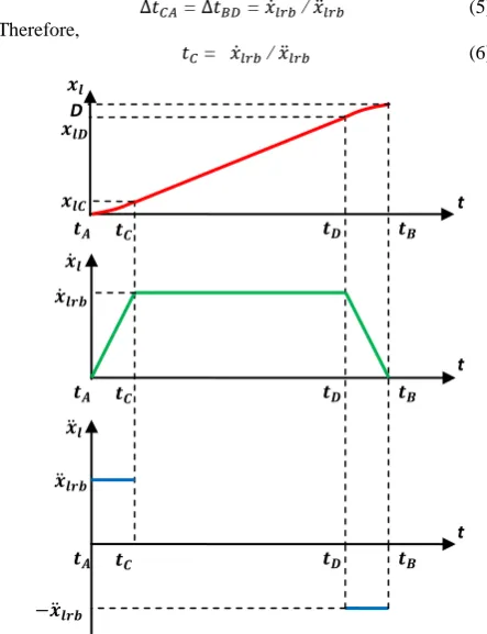
Figure 2 describes the motion along the DP (local coordinates) using 2nd order polynomial. From the velocity diagram in Figure 2, the time intervals and are
given by:
= = / (5) Therefore,
= / (6)
Figure 2: The robot motion along the DP (in Direction)
From the distance diagram in Figure 2, the distance between A and B can be written as:
d = (7)
Substituting (6) into (7) leads to
= = / 2 (8) From the distance diagram in Figure 2,
= D – 2 = ( – 2 ) (9)
By substituting (5) into (9), can be written as:
= D / + / (10)
t
t
t
D
Obstacle 1
Obstacle 2 Obstacle 3
Target B
Starting Point A
DP Robot
o
Obstacle 4
[image:2.595.66.293.295.403.2]
From Figure 2, can be calculated by
= − (11)
Substituting (5) and (10) into (11), leads to
= D / (12)
Therefore,
= − = D / − / (13) Where, D is the distance between points A and B. and
, are the velocity and acceleration of the robot in the
direction.
The motion along the desired path (DP) can be described as follows:
- = dt = dt + dt dt
Therefore; - =
(14)
3.
OBSTACLE AVOIDANCE
The basic strategy of obstacle avoidance is to use the concept of the Configuration Space. The basic idea of Configuration Space or C-Space is to take a robot and its workspace, and reduce the robot to a single point, while expanding the obstacles in the workspace to take account of the shape of the robot. The original workspace is transformed into C-Obstacles and C-Free space. The appeal of this idea is that problems of path-planning or of positioning a robot or object within a workspace are reduced to problems involving a single point. It is easier, for example, to deal with the intersection of a single point with C-Space obstacles, rather than with intersections of obstacles and robot in a Cartesian workspace.
As shown in Figure 3, the radius of an obstacle is expanded to:
= + (15)
Where, is the robot radius, is the radius of an obstacle and is the radius of the expanded obstacle. The robot is
[image:3.595.314.547.217.453.2]then considered as a point. A robot being able to avoid an obstacle is equivalent to the point robot being capable of avoiding the expanded obstacle.
Figure 3: Simplification of the Obstacle
Since the robot rarely uses the back sensors because the robot usually moves forward, the back sensors are excluded in designing the robot. The robot uses six ultrasonic sensors ordered as depicted in Figure 4.
3.1
The sensing vector
The distance of checking collision can be defined as threshold for detecting obstacles. When the obstacle is sensed under this threshold, the value of the sensor will be turned to one (1), otherwise, zero (0). Therefore, the “sensing vector”
which is a binary vector can be defined as follows:
= [LS LMS LFS RFS RMS RS] (16)
Where,
LS refers to Left Sensor, LMS: Left Middle Sensor, LFS: Left Front Sensor, RFS: Right Front Sensor, RMS: Right Middle Sensor, RS: Right Sensor.
Figure 4:The three wheeled omnidirectional robot occupied with six ultrasonic sensors
Each element of the “sensing vector” has either the value of 1 or 0. More than one element can has the value of one. Figure 4 shows an example of detecting many obstacles in the same time.
= [1 0 0 1 1 0 ]
3.2
The gap vector
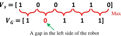
To keep the robot as close as possible to the desired path DP, the robot searches for the existence of gaps between obstacles to pass through them. A “gap” can be defined as the existence of two adjacent zeroes in the “sensing vector”. The “gap vector” is formed from the “sensing vector” by calculating the maximum of each two adjacent elements. The result is a five elements vector which has the form:
= [LG MLG FG MRG RG] (17) Where,
LG: left gap, MLG: Middle left gap, FG: Front gap, MRG: Middle Right gap, RG: Right gap.
In the “gap vector”, the gap is the existence of zero. In the example given in Figure 4, the “gap vector” is constructed as follows:
RS RMS RFS LFS LMS LS
Obstacle
[image:3.595.63.278.602.737.2]Figure 5: An example of constructing the gap vector
It can be seen in the above example that there is a zero on the left side of the vector, which means the existence of a gap on the left side of the robot.
3.3
Distance of Checking Collision
The distance of checking collision can be defined as threshold for detecting obstacles. When the relative distance with all obstacles is longer than , the possibility of collision with obstacles is not checked, and the robot will keep moving on the DP until its relative distance with an obstacle is less than or equal to , where the robot starts checking possible collisions with obstacles.
Assume the maximum velocity of an obstacle in
direction is the same as the maximum speed of the robot . In the case when the obstacle moves towards the robot along the DP (in this case, the distance should the robot pass it
is longer than any distance in any other cases) both at their maximum speed, the relative speed between a robot and an obstacle can be written as:
= − = 2 (18)
If the maximum velocity and acceleration of the robot in the direction are and respectively, the time needed
to move the robot a distance of in the direction can be calculated from the first and the second parts of Equation (14) as follows:
∆t =
(19)
The relative distance between the robot and obstacle that the robot should start to check possible collision is then:
= ∆t (20)
Therefore,
=
(21)
3.4
Avoiding Obstacle in
Direction
When the relative distance with an obstacle is within the range determined by , the robot starts to check possible collisions. It starts to increase (or decrease) the speed in direction if (S = 1), while S is the max of sensing vector elements:
S = Max ( ) (22) Note that S has either the value of one or zero. If S = 1, there is an obstacle detected under the distance of checking collision , if S = 0, no obstacle is detected.
The “gap vector” = [LG MLG FG MRG RG] is constructed from the “sensing vector” . To keep the robot as close as possible to the DP, the robot starts checking the existence of a near gap with FG. If FG = 0, there is a gap at the front of the robot, therefore, the robot keeps its motion (
= 0). If FG = 1, the robot checks the next neighbor gap in the right side (MRG). If MRG = 0, there is a gap in the middle right side of the robot, so, the robot increases its speed in −
direction until it reaches the gap, where the robot speed in direction will be zero ( = 0). If MRG = 1, the robot
checks the next neighbor gap on the left side MLG. If MLG = 0, there is a gap on the left side of the robot, so that the robot increases its speed in + direction until it reaches the gap,
while its speed in direction will be zero. If MLG = 1, the robot checks the last right gap RG. If RG = 0, the robot increases its speed in − direction until it reaches the gap,
where the robot speed in direction will be zero ( = 0),
else, the robot avoids the obstacle in + direction.
Assuming is the acceleration and is the maximum velocity of the robot in the direction; the velocity in the direction can be summarized as follows:
=
–
(23)
3.5
Returning to the
DP
A condition of returning to the DP ( ) which is the
distance between the robot and the desired path DP can be defined as follows:
= − (24) Where and refer to the coordinates of the robot and the
starting point A in direction respectively.
After reaching the position of returning to the DP ( ), the robot starts decrease (or increase) the velocity in direction to return to the DP. is accelerated in the direction of returning to DP. The velocity in the direction after the robot reaches the position of returning to the DP can be written as follows:
=
–
(25)
Where is the sample time.
3.6
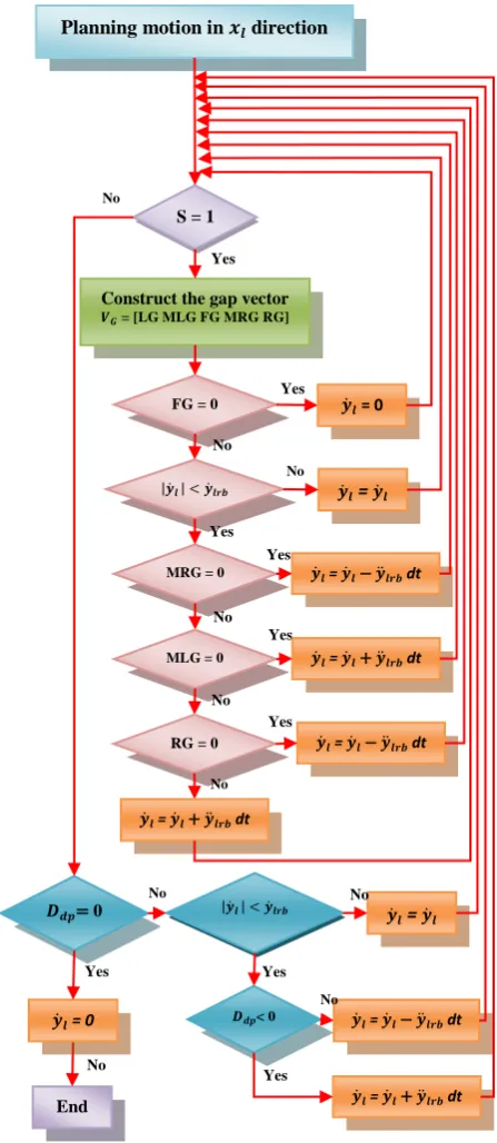
Flowchart of path planning and
obstacle avoidance
Figure 6 gives the flowchart of path planning and obstacle avoidance strategy. First, the robot plans its motion in the direction using Equation (14). If an obstacle appears in the range of checking collision (S = 1), the robot begins to avoid the obstacle in the direction using Equation (23) until it reaches the position of returning to the DP ( ) where, the robot starts to return to the DP using Equation (25).
= [ 1 0 0 1 1 0]
= [ 1
0
1 1 1]
Max
Figure 6: The flowchart of the proposed approach
4.
SIMULATIONS RESULTS
Path planning and obstacle avoidance strategy was simulated using the MATLAB Simulink. The proposed strategy can deal with both static and dynamic obstacles. First, the simulation of the robot’s navigation in the environment with single obstacle in the two cases static and dynamic has been achieved; then the navigation in the environment with multiple obstacles in both cases static and dynamic has been accomplished.
4.1
Single obstacle avoidance
Single obstacle avoidance is simulated in both cases static and dynamic obstacle. The simulation data is given in SI units.
4.1.1
Static single obstacle avoidance
Static obstacle avoidance is achieved as a special case of dynamic obstacle avoidance with zero obstacle velocity. Table 1 gives the data used for static single obstacle avoidance.
Table 1: The data of static single obstacle avoidance
0.1 0.1 1.4 1.4 0.6 1.5 0.7 0.7
Where;
( , ) are the starting point coordinates in the global frame,
( , ) are the target coordinates in the global frame, is the maximum velocity of the robot in direction,
is the acceleration of the robot in direction and
( , ) are the obstacle coordinates in the global frame.
[image:5.595.323.534.360.553.2]The robot is commanded to move from the starting point A(0.1, 0.1) to the target point B(1.4, 1.4) avoiding the obstacle located at (0.7, 0.7) (see Figure 7). The time needed to reach the target is = 3.4641 sec.
Figure 7: Static single obstacle avoidance.
Figure 8 illustrates how the robot uses the “sensing vector” and the “gap vector” to avoid the obstacle of the above example. First, the robot plans its motion toward the target in direction. The robot has continued moving (while S = 0) until the sensor LFS has detected an obstacle (LFS = 1, therefore S = 1), where the robot starts increasing its velocity in direction to reach the nearest gap which is the MRG gap. The robot has continued increasing its velocity until it has reached the maximum velocity. When the robot has reached the gap, the “gap vector” has been changed and a new nearest gap has been appeared at the front (FG = 0), in this case the robot velocity in direction will be zero and the robot keeps its motion until it reaches the condition of returning to the desired path DP (S = 0) where it starts increase its velocity in the direction to the DP (in this case,
direction) until it reaches the DP.
0 0.5 1 1.5
0 0.5 1 1.5
Robot navigation
xG(m) yG
(m)
= 0
S = 1
Construct the gap vector
= [LG MLG FG MRG RG] Yes No
Planning motion in direction
FG = 0 = 0
No Yes
MRG = 0 01
= dt
No Yes
MLG = 0 01
Yes
= + dt
No
RG = 0 Yes
= dt
No
= + dt
End
< 0
= + dt Yes
= dt
No
=
= 0
No No
Yes
Yes
= No
Yes
Figure 8: Illustrating how the robot uses the “sensing vector” and the “gap vector” to avoid the obstacle.
4.1.2
Dynamic single obstacle avoidance
Figure 9 gives the simulation results of dynamic single obstacle avoidance using the data of Table 2. The robot is commanded to move from the starting point A(0.1,0.1) to the destination point B(1.4,1.4) avoiding the obstacle located initially at point (1.3,0.25) which moves with the velocity of 0.5 m/s across the DP with angle of 125°.
Table 2: The data of dynamic single obstacle avoidance
0.1 0.1 1.4 1.4 0.6
1.5 1.3 0.25 0.5 125
Figure 9: Dynamic static single obstacle avoidance simulation.
It can be seen that the robot successfully avoids the obstacle by increasing its velocity in direction to pass before the obstacle.
4.2
Multiple obstacle avoidance
Multiple obstacle avoidance is simulated in both cases static and dynamic obstacles.
4.2.1
Static multiple obstacle avoidance
Static multiple obstacle avoidance is simulated for the case of six obstacles.
Figure 10 shows the simulation result of six static obstacles avoidance using the data of Table 3. The robot starts from point A(0, 0) goes to the target B(2, 2) avoiding six static obstacles located at the positions (0.8, 0.4), (0.8, 0.8), (1, 1.8), (1, 1.4), (1.5, 1.1) and (1.75, 1.75).
Table 3: The data of six static obstacles avoidance
0 0 2 2 0.6 1.5 0.8
0.4 0.8 0.8 1 1.8 1 1.4
1.5 1.1 1.75 1.75
Figure 10: Six static obstacles avoidance simulation.
4.2.2
Dynamic multiple obstacle avoidance
Two cases are simulated, two and six dynamic obstacles. Figure 11 illustrates the simulation result of two dynamic obstacles avoidance, the data of simulation is given in the Table 4. The robot initially located at A(0.1, 0.1) moves toward the target B(2, 2). The first obstacle starts moving from the position (1.8, 0.2) perpendicularly to the DP with velocity of 0.3 m/s and the angle 135°, while the second obstacle starts moving from position (1.7, 1.7) toward the robot with velocity of 0.2 m/s and the angle -135°. The robot successfully avoids the two obstacles by passing between them.
Table 4: The data of two dynamic obstacles avoidance
0.1 0.1 2 2 0.6 1.5 1.8
0.2 0.3 135° 1.7 1.7 0.2 -135°
0 0.5 1 1.5 2
0 0.2 0.4 0.6 0.8 1 1.2 1.4 1.6 1.8 2
Robot navigation
xG(m) yG
(m)
RS RM
S RFS LFS LMS LS
0
0
0
0
0
0 0
0
1
0
0
0 0
1
0
0
0
0 1
0
0
0
0
0
0
0
0
0
0
0 S = 0 S = 1 S = 1 S = 1 S = 0
Note that, refers to the velocity of the obstacle i, while refers to the angle of direction of motion of the obstacle
[image:7.595.318.540.97.302.2]i.
Figure 11: Two dynamic obstacles avoidance simulation.
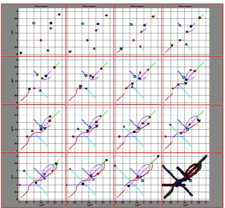
With six dynamic obstacles, the environment will be cluttered and it is difficult for the robot to avoid all the obstacles. Figure 12 shows the robot avoiding the six obstacles successfully. The robot is commanded to move from the starting point A(0.1,0.1) to the destination point B(2,2). The first and the second obstacle are initially at the point (2.8,2.8) and (2.2,2.2) respectively, move toward the robot with a velocity 0.25 m/s and an angle -135°. The third obstacle initially positioned at (2, 0.3) moves with a velocity 0.4 m/s and an angle 135°. The fourth initially is at the position (1, 2.2) moves with a velocity 0.18 m/s and an angle - 45°. The fifth starts from the initial position (1.5, 1) with a velocity 0.25 m/s and an angle -180°. The sixth initially is at the point (2, 2) moves on elliptic path, where its position in and direction is given by the following equations:
(26)
Where,
(27)
(28)
[image:7.595.56.278.111.268.2]The time needed for the simulation is = 7.2354 sec.
Table 5: The data of six dynamic obstacles avoidance
0.1 0.1 2 2 0.6 1.5 2.8
2.8 0.25 -135° 2.2 2.2 0.25 -135°
2 0.3 0.4 135° 1 2.2 0.18
-45° 1.5 1 0.25 -180° 2 2
0.3 -110°
Figure 13 shows how the robot has used the “sensing vector” and the “gap vector” to avoid the six dynamic obstacles. First, the robot has detected a gap on the left side MLG, so that the robot has moved to it. After reaching the gap, the “gap vector” has been changed; the nearest gap is the FG gap and the robot
velocity in direction has become zero. After that, the new nearest gap is the MRG gap, and so on.
Figure 12: Six dynamic obstacles avoidance simulation.
Figure 13: illustrating how the robot uses the “sensing vector” and the “gap vector” to avoid six dynamic
obstacles.
5.
CONCLUSIONS
An autonomous navigation approach for three wheeled omnidirectional mobile robot has been achieved successfully. The navigation based on a hybrid method which combines between a global approach applied to the motion along the desired path (DP) using 2nd order polynomial planning and a local reactive approach used to avoid collisions with static and/or dynamic obstacles based on the “sensing vector” and the “gap vector”. The use of the “gap vector” enables the robot to plan its path in a cluttered environment and to keep its path as close as possible to the desired path (DP) while avoiding obstacles. The simulation results show the effectiveness of this approach. This approach can be improved by incorporating six back sensors to enable the robot to cope with back obstacles, so that the “sensing vector” will have twelve elements. The “sensing vector”, can be extended to the “sensing matrix” which is “3×12” matrix to predict the obstacle motion.Future work should look at this possibility.
RS RMS RFS LFS LMS LS
0
0
0
0
0
0 0
0
0
1
0
0 0
0
0
0
0
1 0
1
1
0
0
0
0
0
0
0
0
0 S = 0 S = 1 S = 1 S = 1 S = 0
MLG
FG
[image:7.595.324.536.336.523.2] [image:7.595.56.280.577.689.2]6.
REFERENCES
[1] M. A. Batalin, G. S. Sukhatme and M. Hattig, Mobile Robot Navigation using a Sensor Network, In IEEE International Conference on Robotics and Automation, New Orleans, LA, pp. 636-642, April 26 - May 1, 2004. [2] W. Hai-hua and L. Dong-liang, obstacle avoidance path
planning in robot soccer, IEEE 2nd Conference on Environmental Science and Information Application Technology, pp. 748-750, 2010
[3] L. Tang ,S. Dian, G. Gu, K. Zhou, S. Wang and X. Feng, A Novel Potential Field Method for Obstacle Avoidance and Path Planning of Mobile Robot, IEEE, 2010. [4] N. H. Viet, N. A. Vien, S. G. Lee, and T. C. Chung,
Obstacle Avoidance Path Planning for Mobile Robot Based on Multi Colony Ant Algorithm, IEEE 1st International Conference on Advances in Computer-Human Interaction, pp. 285-289, 2008.
[5] M. Kam, X. Zhu, and P. Kalata, Sensor Fusion for Mobile Robot Navigation, proceedings of the IEEE, Vol. 85, N° 1, pp. 108-119, January, 1997.
[6] M. O. Franz and H. A. Mallot, Biomimetic robot navigation, Robotics and Autonomous Systems, 30, pp. 133–153, 2000.
[7] P. Bhattacharya and M. L. Gavrilova, Roadmap-Based Path Planning, Using the Voronoi Diagram for a Clearance-Based Shortest Path, IEEE Robotics & Automation Magazine, pp. 58-66, JUNE 2008.
[8] S. Garrido, L. Moreno and D. Blanco, Voronoi Diagram and Fast Marching applied to Path Planning, Proceedings of the IEEE International Conference on Robotics and Automation Orlando, Florida, pp 3049-3054, May 2006. [9] S.S. Keerthi, C.J. Ong, E. Huang, E.G. Gilbert,
Equidistance Diagram - A New Roadmap Method for Path Planning, Proceedings of the IEEE International Conference on Robotics & Automation Detroit, Michigan, pp. 682-687, May 1999.
[10]N. Buniyamin, W. Ngah, N. Sariff and Z. Mohamad, A Simple Local Path Planning Algorithm for Autonomous Mobile Robots, International Journal of Systems Applications, Engineering & Development, Issue 2, Volume 5, pp. 151-159, 2011.
[11]L. Chengqing, M. HAng Jr, H. Krishnan and L. S. Yong, Virtual Obstacle Concept for Local-minimum-recovery in Potential-field Based Navigation, Proceedings of the IEEE International Conference on Robotics & Automation San Francisco, CA, pp. 983-988, April, 2000.
[12]W. H. Huang, B. R. Fajen, J. R. Fink and W. H. Warren, Visual navigation and obstacle avoidance using a steering potential function, Robotics and Autonomous Systems 54, Elsevier, pp. 288–299, 2006.
[13]J. Borenstein, and Y. Koren, Real-time Obstacle Avoidance for Fast Mobile Robots, IEEE Transactions on Systems, Man, and Cybernetics, Vol. 19, No. 5, pp. 1179-1187, Sept/Oct. 1989.
[14]J.Borenstein & Y. Koren, The Vector Field Histogram - Fast Obstacle Avoidance For Mobile Robots, IEEE Transactions on Robotics And Automation, vol. 7, N° 3, pp. 278-288, June 1991.
[15]I. Ulrich and J. Borenstein, VFH+: Reliable Obstacle Avoidance for Fast Mobile Robots, Proceedings of the
1998 IEEE International Conference on Robotics and Automation, Leuven, Belgium, pp. 1572 – 1577, May 16–21, 1998.
[16] I. Ulrich and J. Borenstein, VFH*: Local Obstacle Avoidance with Look-Ahead Verification, IEEE International Conference on Robotics and Automation, San Francisco, CA, pp. 2505-2511, April 24-28, 2000. [17] Y. Cang and J. Borenstein, A Method for Mobile Robot
Navigation on Rough Terrain, IEEE International Conference on Robotics and Automation, New Orleans, LA, pp. 3863-3869, April 26-May 1, 2004.
[18] J. Minguez and L. Montano, Nearness Diagram (ND) Navigation: Collision Avoidance in Troublesome Scenarios, IEEE Transactions On Robotics And Automation, Vol. 20, N°. 1, pp. 45-59, February 2004. [19] S. Khatoon and Ibraheem, Autonomous Mobile Robot
Navigation by Combining Local and Global Techniques, International Journal of Computer Applications, Volume 37, N° 3, January 2012.
[20] H. Teimoori and A V. Savkin, Equiangular Navigation Guidance of a Wheeled Mobile Robot with Local Obstacle Avoidance, Proceedings of the IEEE International Conference on Robotics and Biomimetics, Bangkok, Thailand, pp.1962-1967, February 21 - 26, 2008.
[21] Y. Jincong, Z. Xiuping, N. Zhengyuan, H. Quanzhen, Intelligent Robot Obstacle Avoidance System Based on Fuzzy Control, The IEEE 1st International Conference on Information Science and Engineering (ICISE), pp. 3812-3815, 2009.
[22] C. Cai1, C. Yang, Q. Zhu and Y. Liang, A Fuzzy-based Collision Avoidance Approach for Multi-robot Systems, Proceedings of the IEEE International Conference on Robotics and Biomimetics, Sanya, China, pp. 1012-1017, December 15 -18, 2007.
[23] V. Yadav, X. Wang and S.N. Balakrishnan, Neural Network Approach for Obstacle Avoidance in 3-D Environments for UAVs, Proceedings of the American Control Conference Minneapolis, Minnesota, USA, pp. 3667-3672, June 14-16, 2006.
[24] J. A. F. Leon, M. Tosini and G. G Acosta, Evolutionary Reactive Behavior for Mobile Robots Navigation, Proceedings of the IEEE Conference on Cybernetics and Intelligent Systems, Singapore, pp. 532-537, 1-3 December, 2004.
[25] D. R. Parh, J. K. Pothal and M. K. Singh, Navigation of Multiple Mobile Robots Using Swarm Intelligence, World Congress on Nature & Biologically Inspired Computing (NaBIC), pp. 1145-1149, 2009.
[26] R. R. Sahoo, P. Rakshit and M. T. Haidar, Navigational Path Planning of Multi-Robot using Honey Bee Mating Optimization Algorithm (HBMO), International Journal of Computer Applications, Volume 27, No.11, August 2011.