12
Classification of Moving Vehicles using Multi-Classifier
with Time-Domain Approach
N. Abdul Rahim
Universiti Malaysia Perlis School of Mechatronic Eng.Pauh Putra Campus
Paulraj M P
Universiti Malaysia Perlis School of Mechatronic Eng.Pauh Putra Campus
A.H. Adom
Universiti Malaysia Perlis School of Mechatronic Eng.Pauh Putra Campus
ABSTRACT
The hearing impaired is afraid of walking along a street and living a life alone. Since, it is difficult for hearing impaired to hear and judge sound information and they often encounter risky situations while they are in outdoors. The sound produced by moving vehicle in outdoor situation cannot be moderated wisely by profoundly hearing impaired community. They also cannot distinguish the type and the distance of any moving vehicle approaching from their behind. In this paper, a simple system that identifies the type and distance of a moving vehicle using artificial neural network has been proposed. The noise emanated from a moving vehicle along the roadside was recorded together with its type and position. Using time-domain approach, simple feature extraction algorithm for extracting the feature from the noise emanated by the moving vehicle has been developed. Simple time-domain features such as energy and zero-crossing rates are applied for getting the important signatures from the sound. The extracted features were associated with the type and zone of the moving vehicle and a multi-classifier system (MCS) based on neural network model has been developed. The developed MCS is tested for its validity.
General Terms
Pattern Recognition, Moving Vehicle, Multilayer Perceptron
Keywords
Multi-Classifier, Time-Domain, Voting System
1.
INTRODUCTION
Acoustic noise signature emanated from moving vehicle along the roadside is mainly influenced by the engine vibration and the friction between the tires and the road. The vehicle of the same type and working in a similar condition will posses almost similar noise signature [1]. This pattern of noise signature is used for classifying the type of vehicle and their distance from the subject.
Recently, a number of studies have been done on sound signature analysis of moving vehicle. Henryk Maciejewski et. al. [2] developed a neural classifier to classify the type of a moving vehicle based on the noise produced by engine and carriageable devices. Wavelet method has been used for feature extraction. Similar features extraction method has been made by Amir Averbuch [3, 4]. Huadong Wu et. al. [1] proposed a frequency vector principle to recognize the moving vehicle based on its sound signature. Eom [5], using time-varying autoregressive models expanded by a low-order discrete cosine transform classified the type of moving vehicles. Bayesian subspace methods based on the short term Fourier transform has been proposed by Munich [6] to recognize the type of the moving vehicle. A simple approach
based on nonlinear Hebbian learning has been implemented by Bing Lu et. al. [7] to classify the type of moving vehicles.
Based on literature, it has been observed that most of the authors have dealt only with the recognition of the vehicle types. The distance between the hearing impaired and the approaching vehicle from their behind is a very important criterion and this criterion has not been considered by early researchers. Hence, in this research work, a simple scheme has been proposed to identify the type as well as the distance of the moving vehicles based on the noise emanated by them. The maximum distance from the subject to the moving vehicle is considered as 100 meters. When the moving vehicle is approaching the subject from a distance of 100 meters, the noise emanated from the vehicle is continuously recorded till it crosses the observer. The energy, zero-crossing rate and statistical values were extracted and associated to the type and distance of the moving vehicle. The developed feature set was then used to model a feedforward network trained by Levenberg-Marquardt algorithm.
2.
METHODOLOGY
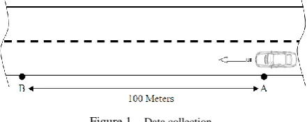
The noise emanated from a moving vehicle is recorded using a digital voice recorder (ICD-SX700). The recording was carrying out along the section of road from Ulu Pauh to Padang Besar. The average speed of the vehicles along this road is between 50 – 70 km/h. Two different locations along the section of the road were considered and marked as A and B as shown in Figure 1. The distance between the locations A and B is 100 meters. The digital sound recorder is placed at point B. The noise emanated from a vehicle was continuously recorded as it was traversing towards the point B from the point A. The time taken by the vehicle to traverse the distance AB was also observed. The recording was carried out under normal wind condition.
Figure 1. Data collection
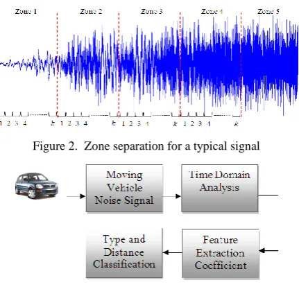
[image:1.595.320.541.596.684.2]13 obtained using time-domain analysis. These coefficient values
[image:2.595.61.277.137.344.2]were than associated to the respective zone number as well as to the type of vehicle and used to develop a multiple classifier system (MCS) based neural network model. The model was trained using Levenberg-Marquardt algorithm. The complete type and zone classification system is depicted in Figure 3.
Figure 2. Zone separation for a typical signal
Figure 3. Block diagram of a moving vehicle classification system
3.
FEATURE EXTRACTION
The recorded noise signal from each zone is divided into frames such that each frame has 1024 samples. Frame overlapping is not considered in this analysis. For each frame, time-domain features namely short-time energy (STE), low short-time frame energy ratio (LSTFER), change of energy, energy variation, zero-crossing rate (ZCR) and high frame zero-crossing rate ratio (HFZCRR) are computed. The basic statistical features namely standard deviation, average, median, variance, kurtosis and skewness were also computed
3.1
Short Time Energy (STE)
The amplitude of the noise emanated from a moving vehicle varies with time. The energy level of the noise is reflected in its amplitude. The STE corresponding to an mth frame is
computed using the following equation [8, 9].
2 2 1,
N
n n
n
STE m x w
m1, 2,3,...,k (1)where N is the number of samples in the mth frame, xn is the
nth frame signal and wn is a window function. The rectangular
window (wn = 1) has been chosen in this analysis [10].
After computing the STE for all the frames, the change in short-time energy is computed using Equation 2.
( ) 1 ,
STE m STE m STE m
m1, 2,3,...,k1 (2)
The short-time energy variation between any two consecutive frames is computed using Equation 3.
( ) 1 * 1 ,
V
STE m STE m STE m STE m STE m
(3)
1, 2,3,..., 1
m k
Low short-time frame energy ratio (LSTEFR) is defined as the number of signals in a frame where the energy level of the signal is less than fifty percent of the overall average signal energy for the whole frame. LSTEFR is computed using the relation shown in Equation (4).
1 1
( ) 0.5 * 1
2
N
n n
n
LSTER m sign X x x
N
(4)where,
1
1 N n n n
X x x
N
3.2
Short Time Zero-Crossing Rate
Short Time Zero-Crossing Rate (STZCR) occurs, if successive STE waveform samples have different algebraic sign [11]. Using sign functions STZCR can be computed as shown in Equation (5).
1 11 2
N
n n n
n
STZCR m sign x sign x w
(5)The high frame zero-crossing rate ratio (HFZCRR) can be defined as a number of signal whose energy level is greater than 1.5 times the average energy signal of the frame. Using Equation 6, the HFZCRR can be computed.
1 1
( ) * 1.5 1
2
N
n n
n
HFZCRR n sign x x X
N
(6)where,
1
1 N
n n
n
X x x
N
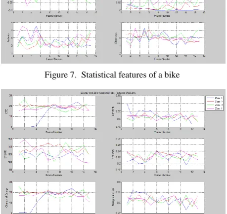
[image:2.595.312.545.447.583.2]The developed feature set was then used to model a multi-classifier system based on feedforward network trained by Levenberg-Marquardt algorithm. The typical time-domain features of a car, bike, lorry and truck were depicted in Figure 4 to 11 respectively.
[image:2.595.314.542.608.748.2]Figure 4. Energy and zero-crossing rate features of a car
14 Figure 6. Energy and zero-crossing rate features of a bike
[image:3.595.54.283.233.379.2]Figure 7. Statistical features of a bike
Figure 8. Energy and zero-crossing rate features of a lorry
Figure 9. Statistical features of a lorry
Figure 10. Energy and zero-crossing rate features of a truck
Figure 11. Statistical features of a truck
4.
MULTI-CLASSIFIER SYSTEM
For the classification of vehicle type and zone, multi-classifier systems (MCS) have been employed. A MCS was formulated by combining several different base network classifiers. As the classification accuracy of a single classifier is less during testing phase, a MCS is used. A MCS contains number of sub classifiers (C1, C2,…,Cn). Each sub classifier is modeled using a portion of the training data base. These sub classifier models were then combined using a simple fusion algorithm to yield the correct classification type. The architecture of a parallel [12, 13] MCS is shown in Figure 12.
Figure 12. Architecture of a parallel MCS
[image:3.595.315.544.237.378.2] [image:3.595.53.283.306.523.2] [image:3.595.321.569.528.682.2] [image:3.595.54.281.558.698.2]15 It also inherits the intelligence and nonlinear characteristic of
the brain. The general structure of multilayer perceptron neural network is shown in Figure 13. Levenberg-Marquardt training algorithm is used to train the data set since it takes less training time [16]. In this paper, a neural network model is used as a base classifier for the MCS.
Figure 13. Multilayer perceptron neural network
4.2
Fusion
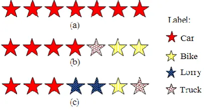
To classify the output class label, majority voting fusion [12, 17] has been employed in this research work. Majority voting fusion has three voting schemes namely, unanimity voting, simple majority voting and plurality voting. For unanimity or majority voting the decision will be made only if all the output form base classifier returns the same class label. Meanwhile, simple majority voting will produce the result when the base classifier output given at least one more than half the number of classifiers give a same class label and plurality voting will give the output when the base classifier give the highest number of votes, whether or not the sum is exceed 50%. The three voting patterns are illustrated in Figure 14.
Figure 14. Voting System (a) Unanimity (b) Simple Majority and (c) Plurality
5.
RESULT AND DISCUSSION
[image:4.595.57.291.142.273.2]Four different types of vehicles namely car, bike, truck and lorry are considered in this research. Table 1 depicts the number of vehicles observed and used in the analysis.
Table 1. Table captions should be placed above the table
Type of Vehicle Sample
Car 35
Bike 35
Lorry 35
Truck 35
Total 140
The noise signal recorded is separated into frames such that each frame has 1024 samples. From each frame, 12 features
namely time energy, change in time energy, time energy variation, low time frame energy ratio, short-time zero-crossing rate, high frame zero-crossing rate ratio, standard deviation, average, median, variance, kurtosis and skewness were extracted. The number of frames for each zone varies as it depends on the speed of the moving vehicle traversing from point A to point B. Features from three consecutive frames were combined together and the combined 36 features were associated to the vehicle type. The method of combining three consecutive frames is depicted in Figure 15. This process was repeated for the entire 140 recorded signal and a data set containing of 10680 samples was formulated.
Figure 15. Features from consecutive frame
The data set is randomized and normalized between -0.9 to +0.9. Initially 50% of the samples were selected at random from the main data set. Using the randomly selected sampled data set, a neural network was modeled to associate the 36 time-domain features with the type of the vehicle. The developed network model was tested with remaining feature samples. The above analysis was repeated by selecting 60%, 70% and 80% of the samples randomly from the data set as training data sets. Four different neural network models were developed and the classification accuracies are show in Table 2. From Table 2, it can be observed that the testing classification accuracy of the models is below 68%. The 80% training data set has a better result when compared with the other neural network models.
As the classification accuracy of the vehicle type classification network model using single classifier is less MCS was applied. The data set for each base classifier was selected randomly from the main data set. As the neural network model developed using 80% of the data samples give a better result, 80% of the samples were chosen at random from the main data set and a base classifier data set was formulated. For each base classifier data set, a neural network model was developed to classify the vehicle type and their classification accuracies were determined. The classification accuracy of the base classifier network models are shown in Table 3. After formulating the subset classifier models, combining classifiers was applied and the network classification accuracy was determined and shown in Table 3.
[image:4.595.314.550.203.301.2] [image:4.595.65.269.449.558.2]16 A similar procedure was repeated and MCS network models
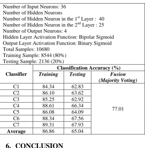
were developed to identify the vehicle zone. The classification results for the developed MCS network models are shown in Tables 4 and 5. From Table 4, it can be observed that the neural network model trained using 80% data samples has better classification accuracy when compared to the other neural network models. Then, 80% of the samples were chosen at random from the main data set and a base classifier data set was formulated. For each base classifier data set, a neural network model was developed to classify the vehicle zone and their classification accuracies were determined. The classification accuracy of the base classifier network models are shown in Table 5. After formulating the subset classifier models, combining classifiers was applied and the network classification accuracy was determined and shown in Table 5. From Table 5, seven out of thirty base classifiers have been formulated. Further, it can be observed in Table 5 that the average training classification accuracy is 86.86%. The subset models were tested with remaining data samples and the average classification accuracy is 65.04%. Applying the parallel MCS voting system the classification accuracy is 77.01%. The proposed MCS has improved the vehicle type classification accuracy by 11.97%.
Table 2. classification accuracy for vehicle type using single classifier
Number of Input Neurons: 36 Number of Hidden Neurons
- Number of Hidden Neuron in the 1st Layer : 40 - Number of Hidden Neuron in the 2nd Layer : 25 Number of Output Neurons: 4
Hidden Layer Activation Function: Bipolar Sigmoid Output Layer Activation Function: Binary Sigmoid Total Samples: 10680
Data Sample (%)
Classification Accuracy (%) Training Testing
50 89.93 61.27
60 88.96 62.33
70 86.75 64.32
[image:5.595.306.552.305.557.2]80 86.90 67.14
Table 3. Classification accuracy for vehicle type using MCS
Number of Input Neurons: 36 Number of Hidden Neurons
- Number of Hidden Neuron in the 1st Layer : 40 - Number of Hidden Neuron in the 2nd Layer : 25
Number of Output Neurons: 4
Hidden Layer Activation Function: Bipolar Sigmoid Output Layer Activation Function: Binary Sigmoid Total Samples: 10680
Training Sample: 8544 (80%) Testing Sample: 2136 (20%)
Classifier
Classification Accuracy (%) Training Testing Fusion
(Majority Voting)
C1 83.15 66.01
78.18
C2 87.11 65.36
C3 86.59 67.70
C4 89.96 69.94
C5 84.35 64.98
C6 87.52 67.18
C7 87.48 65.50
Average 86.59 66.67
Table 4. Classification accuracy for vehicle zone using single classifier
Number of Input Neurons: 36 Number of Hidden Neurons
- Number of Hidden Neuron in the 1st Layer : 40 - Number of Hidden Neuron in the 2nd Layer : 25 Number of Output Neurons: 4
Hidden Layer Activation Function: Bipolar Sigmoid Output Layer Activation Function: Binary Sigmoid Total Samples: 10680
Data Sample (%)
Classification Accuracy (%) Training Testing
50 89.65 57.87
60 87.64 60.67
70 87.14 62.86
80 87.13 65.07
Table 5. Classification accuracy for vehicle zone using MCS
Number of Input Neurons: 36 Number of Hidden Neurons
- Number of Hidden Neuron in the 1st Layer : 40 - Number of Hidden Neuron in the 2nd Layer : 25
Number of Output Neurons: 4
Hidden Layer Activation Function: Bipolar Sigmoid Output Layer Activation Function: Binary Sigmoid Total Samples: 10680
Training Sample: 8544 (80%) Testing Sample: 2136 (20%)
Classifier
Classification Accuracy (%) Training Testing Fusion
(Majority Voting)
C1 84.34 62.83
77.01
C2 86.10 63.62
C3 85.25 62.92
C4 88.61 66.34
C5 86.08 64.09
C6 88.34 67.56
C7 89.31 67.93
Average 86.86 65.04
6.
CONCLUSION
The feature sets from time-domain analysis were used to evaluate the type and zone of the moving vehicles. The MCS based neural network model trained by Levenberg-Marquardt algorithm was presented. From experimental results it is inferred that the type and distance of moving vehicle can be identified using the proposed method. As a future research work, it is proposed to design the MCS using different types of network classifiers and different features for each base classifier.
7.
ACKNOWLEDGMENTS
[image:5.595.45.289.342.754.2]17
8.
REFERENCES
[1] W. Huadong, M. Siegel, and P. Khosla, "Vehicle sound signature recognition by frequency vector principal component analysis," in Instrumentation and Measurement Technology Conference, 1998. IMTC/98. Conference Proceedings. IEEE, 1998, pp. 429-434 vol.1. [2] H. Maciejewski, J. Mazurkiewicz, K. Skowron, and T.
Walkowiak, "Neural Networks for Vehicle Recognition," in Proceeding of the 6th International Conference on Microelectronics for Neural Networks, Evolutionary and Fuzzy Systems, 1997, p. 5.
[3] A. Averbuch, E. Hulata, V. Zheludev, and I. Kozlov, "A Wavelet Packet Algorithm for Classification and Detection of Moving Vehicles," Multidimensional Systems and Signal Processing, vol. 12, pp. 9-31, 2001. [4] A. Averbuch, V. A. Zheludev, N. Rabin, and A. Schclar,
"Wavelet-based acoustic detection of moving vehicles," Multidimensional Systems and Signal Processing, vol. 20, pp. 55-80, 2009.
[5] K. B. Eom, "Analysis of Acoustic Signatures from Moving Vehicles Using Time-Varying Autoregressive Models," Multidimensional Systems and Signal Processing, vol. 10, pp. 357-378, 1999.
[6] M. E. Munich, "Bayesian Subspace Methods for Acoustic Signature Recognition of Vehicles," in Proceeding of the 12th European Signal Processing Conference, 2004, pp. 1-4.
[7] L. Bing, A. Dibazar, and T. W. Berger, "Nonlinear Hebbian Learning for noise-independent vehicle sound recognition," in Neural Networks, 2008. IJCNN 2008. (IEEE World Congress on Computational Intelligence). IEEE International Joint Conference on, 2008, pp. 1336-1343.
[8] E. Alexandre, L. Cuadra, L. Álvarez, M. Rosa-Zurera, and F. López-Ferreras, "Automatic Sound Classification for Improving Speech Intelligibility in Hearing Aids
Using a Layered Structure," in Intelligent Data Engineering and Automated Learning – IDEAL 2006, 2006, pp. 306-313.
[9] E. Alexandre-Cortizo, M. Rosa-Zurera, and F. Lopez-Ferreras, "Application of Fisher Linear Discriminant Analysis to Speech/Music Classification," in Computer as a Tool, 2005. EUROCON 2005.The International Conference on, 2005, pp. 1666-1669.
[10]S. Sampan, "Neural Fuzzy Techniques in Vehicle Acoustic Signal Classification," in Faculty of the Virginia Polytechnic Institute and State University, 1997, p. 172.
[11]L. Rabiner and R. Schafer, Theory and Applications of Digital Speech Processing Prentice Hall, 2010.
[12]L. Kuncheva, Combining Pattern Classifiers: Methods and Algorithms: Wiley-Interscience, 2004.
[13]R. Romesh and P. Vasile, "Multi-Classifier Systems: Review and a roadmap for developers," Int. J. Hybrid Intell. Syst., vol. 3, pp. 35-61, 2006.
[14]N. A. Rahim, M. P. Paulraj, A. H. Adom, and S. Sundararaj, "Moving Vehicle Noise Classification using Backpropagation Algorithm," in 2010 6th International Colloquium on Signal Processing & Its Applications, 2010, p. 6.
[15]S. N. Sivanandam and M. Paulraj, Introduction to Artificial Neural Networks: VIKAS Publishing House Pvt Ltd, India, 2003.
[16]N. A. Rahim, M. N. Taib, A. H. Adom, and M. Y. Mashor, "The NARMAX Model for a DC Motor using MLP Neural Network," in Proceeding of the First International Conference 0n MAN-MACHINE SYSTEMS (ICoMMS), 2006, pp. 61-65.