Cusp Catastrophe Polynomial Model: Power and Sample Size Estimation

http://dx.doi.org/10.4236/ojs.2014.410076

Cusp Catastrophe Polynomial Model: Power

and Sample Size Estimation

Ding-Geng Chen

1,2,3

_{, Xinguang Chen}

4,5

_{, Feng Lin}

1,6

_{, Wan Tang}

2

_{, Yuhlong Lio}

7

_,

Yuanyuan Guo

8

1_{Center of Research, School of Nursing, University of Rochester Medical Center, Rochester, NY, USA} 2_{Department of Biostatistics and Computational Biology, University of Rochester Medical Center, Rochester,} NY, USA

3_{Institute of Data Sciences, University of Rochester, Rochester, NY, USA} 4_{Department of Epidemiology, University of Florida, Gainesville, FL, USA} 5_{School of Public Health, Wuhan University, Wuhan, China}

6_{AD-CARE, Department of Psychiatry, University of Rochester Medical Center, Rochester, NY, USA} 7_{Department of Mathematical Sciences, University of South Dakota, Vermillion, SD, USA}

8_{Department of Statistics, Central South University, Changsha, China} Email: din_chen@urmc.rochester.edu

Received 6 October 2014; revised 26 October 2014; accepted 8 November 2014

Copyright © 2014 by authors and Scientific Research Publishing Inc.

This work is licensed under the Creative Commons Attribution International License (CC BY). http://creativecommons.org/licenses/by/4.0/

Abstract

Guastello’s polynomial regression method for solving cusp catastrophe model has been widely ap-plied to analyze nonlinear behavior outcomes. However, no statistical power analysis for this modeling approach has been reported probably due to the complex nature of the cusp catastrophe model. Since statistical power analysis is essential for research design, we propose a novel method in this paper to fill in the gap. The method is simulation-based and can be used to calculate statis-tical power and sample size when Guastello’s polynomial regression method is used to do cusp catastrophe modeling analysis. With this novel approach, a power curve is produced first to depict the relationship between statistical power and samples size under different model specifications. This power curve is then used to determine sample size required for specified statistical power. We verify the method first through four scenarios generated through Monte Carlo simulations, and followed by an application of the method with real published data in modeling early sexual initiation among young adolescents. Findings of our study suggest that this simulation-based power analysis method can be used to estimate sample size and statistical power for Guastello’s polynomial regression method in cusp catastrophe modeling.

Keywords

Determination

1. Introduction

Popularized in the 1970’s by Thom [1], Thom and Fowler [2], Cobb and Ragade [3], Cobb and Watson [4], and Cobb and Zack [5], catastrophe theory was proposed to understand a complicated set of behaviors including both gradual and continuous changes and sudden and discrete or catastrophical changes. Computationally, there are two directions to implement this theoretical catastrophe theory. One direction is operationalized by Guastello

[6] [7] with the implementation into a polynomial regression approach and another direction by a stochastic cusp catastrophe model from Cobb and his colleagues [5] with implementation in an R package in [8]. And this paper is to discuss the first direction on polynomial cusp catastrophe regression model due to its relative simplicity and ease for implementation as simple regression approach. This model has been used extensively in research. Typ-ical examples include modeling of accident process [7], adolescent alcohol use [9], changes in adolescent sub-stance use [10], binge drinking among college students [11], sexual initiation among young adolescents [12], nursing turnover [13], and effect of HIV prevention among adolescents [12] [14].

Even though this polynomial regression method has been widely applied in behavioral studies to investigate the existence of cusp catastrophe, to the best of our knowledge, no reported research has addressed the determi-nation of sample size and statistical power for this analytical approach. Statistical power analysis is an essential part for researchers to efficiently plan and design a research project as pointed out in [15]-[17]. To assist and enhance application of the polynomial regression method in behavioral research, this paper is aimed to fill this method gap by reporting the Monte-Carlo simulation-based method we develope to conduct power analysis and to determine sample size.

The structure of the paper is as follows. We start with a brief review of the cusp catastrophe model (Section 2), followed by reporting our development of the novel simulation-based approach to calculate the statistical power (Section 3). This approach is then verified through Monte Carlo simulations and is further illustrated with data derived from published study (Section 4). Conclusions and discussions are given at the end of the paper (Section 5).

2. Cusp Catastrophe Model

2.1. Overview

The cusp catastrophe model is proposed to model system outcomes which can incorporate the linear model with extension to nonlinear model along with discontinuous transitions in equilibrium states as control variables vary. According to the catastrophe systems theory [1] [18]-[20], the dynamics for a cusp system outcome is expressed by the time derivative of its state variable (often called behavioral variable within the context of catastrophe theory) to the potential function: V z x y

(

; ,

)

=1 4z4−1 2z y2 −zx The first derivative of V will consist of the equilibrium plane of the cusp catastrophe:

(

)

3

, , 0

V z x y z z yz x

∂ ∂ = − − = (1)

where

x

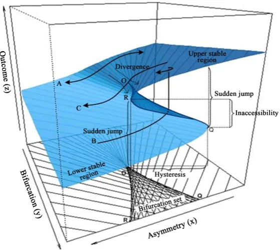
is called asymmetry or normal control variable and y is called bifurcation or splitting control vari-able. In the model, the two control variables x and y co-vary to determine the behavior outcome variable z.

Figure 1 depicts the equilibrium plane which reflects the response surface of the outcome measure

( )

z at var-ious combinations of x and y. It can be seen from the figure that the dynamic changes in a behavior measure

( )

z has two stable regions (attractors), the lower area in the front left and the upper areas in the front right. Beyond these two regions, behavior z becomes unstable. This characteristic can be further revealed by pro-jecting the unstable region to the

x

and y control plane as a cusp region. The cusp region is characterized by two lines, line O-Q (the ascending threshold) and line O-R (the descending threshold) of the equilibrium surface. In this region, the outcome measure becomes highly unstable, and sudden change or jumping in behavior status will occur, because a very small change in x or y or both will lead z to cross either the threshold line O-Q or O-R.

[image:3.595.160.440.85.334.2]

Figure 1. Cusp catastrophe model for outcome measures

( )

Z in the

equili-brium plane with asymmetry control variable

( )

X and bifurcation control

variable

( )

Y . (Annotated by the authors with the original graph produced by Grasman’s R package “cusp”).

outcome measure

( )

z . Path A shows that in any situations where y<O, there is a smooth relation between outcome measure

( )

z and the asymmetry variable

( )

x ; path B shows that in any situations where y>O, if the asymmetry variable x increases to reach and pass the ascending threshold link O-Q, outcome measure

( )

z will increase suddenly from the low stable region to the upper stable region of the equilibrium plane; and Path C shows a sudden drop in outcome measure

( )

z as x declines to reach and pass the descending thre-shold line O-R .

From the affirmative description, it is clearly that a cusp model differs from a linear model in that: 1) A cusp model allows the forward and backward progression follows different paths in the outcome measure and both processes can be modeled simultaneously (see Paths B and C in Figure 1) while a linear model only permits one type of relationship; 2) A cusp model covers both a discrete component and a continuous component of a beha-vior change while a linear model covers on continuous process (Path A). In this case a linear model can be con-sidered as a special case of the cusp model; 3) A cusp model consists of two stable regions and two thresholds for sudden and discrete changes. Therefore, the application of the cusp modeling will advance the linear ap-proach and better assist researchers to describe the behavior data while evidence obtained from such analysis, in turn, can be used to advance theories and models to better explain a behavior.

2.2. Guastello’s Cusp Catastrophe Polynomial Regression Model

To operationalize the cusp catastrophe model for behavior research, Guastello [6] [7] developed the polynomial regression approach to implement the concept of cusp model. Since the first publication of this method, it has been widely used in analyzing real data as we described in the Introduction. In this study, we referred the me-thod as Gastello’s polynomial cusp regression. According to Gustello, this approach is derived by inserting re-gression β coefficients into the Equation (1), with change scores ∆ =z z₂−z₁ (the differences in the mea-surement scores of a behavior assessed at time 1 and time 2) as a numerical approximation of dz:

3 2

0 1 1 2 1 3 1 4 5

z β β z β z β y z β x β y ε

where β₀ is the intercept and

ε

is the normally distributed error term. Two additional term 2

2 z1

β × and

5 y

β × are added to capture potential deviations of the data from the equilibrium plane. When conducting mod-eling analysis, a cusp is indicated ONLY if the estimated β₁ for the cubic term, plus β₃ (for the interaction term) or β₄ (for control variable x) in Equation (2) are statistically significant.

To demonstrate the efficiency of the polynomial regression approach in describing behavioral changes that are cusp, Guastelly [7] recommended a comparative approach. In this approach, two types, four alternative li-near models can be constructed and used in modeling the same variables:

1) Change scores linear models

0 1 1 4 5

z β βz β x β y

∆ = + + + (3)

0 1 1 3 1 4 5

z β βz β yz β x β y

∆ = + + + + (4)

2) Pre-and post-linear models

2 0 1 1 4 5

z =β +β z +β x+β y (5)

2 0 1 1 3 1 4 5

z =β +βz +β yz +β x+β y (6)

These alternative linear models add another analytical strategy to strength the polynomial regression method. A better data-model fitting (or a larger R2) of the cusp model (2) than the alternative linear models (3) through (6) is often used as additional evidence supporting the hypothesis that the dynamics of a study behavior follows the cusp catastrophe. Fitting Guastello’s cusp regression model and the four alternative models can all be con-ducted with commonly available statistical software, including SAS, SPSS, STATA and R. More recent dis-cussions and applications of the cusp catastrophe modeling methods can be found in [21].

3. Simulation-Based Power Analysis Approach for Guastello’s Cusp Regression

3.1. A Brief Introduction to Statistical Power

In statistics, power is defined as the probability of correctly rejecting the null hypothesis. Stated in common language, power is the fraction of the times that the specified null-hypothesis value will be rejected from statis-tical tests. Operationally based on this definition, if we specify an alternative hypothesis H₁, a desired type-I error rate α , and a desired power

(

1−β

)

, then we can calculate the required sample size

n

. Alternatively, we can calculate the statistical power

(

1−β

)

as a function of sample size

n

under a specified alternative hypothesis H₁ and a desired type-I error rate α. There are extensive literatures on sample size calculation as well as statistical power analysis, see the seminal books from [15]-[17] for power analysis for behavioral sciences.

As detailed in Chapter 7 in [17], five factors related to research design interplay with each other to determine the statistical power and sample size for a simple t-test: 1) the rate of type-I error

α

; 2) the desired statistical power 1−β, 3) the expected treatment effect size of δ , 4) the standard error s2 for the expected effect size, and 5) the sample size

n

. The mathematical formula can then be derived as

(

2 2

)

2

1 1

2

n≥ s δ _z_−α+z_−β_ . Therefore, to determine the required sample size

n

, we would need to provide data for four of the five design characteristics. Typically, the type-I error α _{is set at 0.05 and the desired power}

(

1−β

)

is chosen to be 0.85 (or 0.80). The other two will be treatment effect size δ and its standard error s2. Depending on actual re-search questions, different values are often selected for these two characteristics.

Extending the same concept described above for Guastello’s polynomial cusp regression, we would need to specify the corresponding parameter effect size for all βs in Equation (2), the standard deviation of the error term ε. In addition, we need to specify the distribution of the two control variables, the asymmetry x and the bifurcation y; and the distribution of the outcome variable z at time 1 (i.e. z₁). With these parameters and variables being specified, the required sample size for a significant Cuastello’s cusp regression model can be determined and statistical power can be analyzed.

( )

x or the bifurcation variable

( )

y if they are linked to multiple regressors or even to the overall goodness- of-fit index of R2. However, we aim to tackle a more complicated problem to determine whether we can detect a significant overall cusp model. The complexity of cusp catastrophe model makes it rather challenging, if not impossible to derive an analytical formula to determine the statistical power for Guastello’s cusp regression. To deal with this difficult, we propose a Monte-Carlo simulation-based approach. In this method the statistical power is calculated as the fraction of the times that the specified null-hypothesis of “no cusp” is rejected at the given level of type I error. Stated in another way, if there is a cusp, the statistical power will be, among 100 si-mulations, how many times can we detect the cusp given the sample size and type I error? The detailed steps of the simulation-based approach are outlined as follows:

1) Simulate data with sample size

( )

n (i.e. the number of observations for Guastello’s cusp regression mod-eling) for the asymmetry variable x, bifurcation variable y and outcome variable at time 1 (i.e. z₁). Data are generated under required specifications for desired study, such as normal distribution with specific means and standard deviations. Guastello’s cusp regression requires that all variables be standardized before data analysis and modeling. In this case, the standard normal distribution can be used to generate data for

x

,

y and z₁;

2) Specify model parameter effect size β =

(

β β β β β β₀, ₁, ₂, ₃, ₄, ₅

)

and the standard deviation σ of the error term of

ε

(Equation (2)) obtained from prior knowledge;

3) Calculate z₂= +z₁ β₀+β_{1 1}z3+β_{2 1}z2+β₃yz₁+β₄x+β₅y+ε using the data obtained in the previous two

Steps. Also generate ∆ =z z₂−z₁;

4) Fit the Guastello’s cusp regression model (Equation (2)) with least squares method using the data generated for ∆z, x, y, and z₁. After model fitting, a significant test is conducted to determine whether the data fit Guastello’s cusp regression model satisfactorily according to the decision rules proposed by Guastello (1982): 1) the estimated β₁ for the cubic term and 2) β₃ (for the y and z₁ interaction term) or β₄ (for control variable

x

) must be are statistically significant;

5) Repeat Steps 1 to 4 a large number of times (typically 1000) and calculate the proportion of simulations which satisfy the Guastello’s decision rules. This proportion then provides an estimate of the statistical pow-er for the pre-specified sample size and the study specifications given in Steps 1 and 2;

6) With the above established five steps for power assessment, sample size is then determined to reach a pre-specified level of statistical power. This is carried out by running Steps 1 to 5 with a range of sample sizes

( )

n first to obtain the corresponding values of statistical power. Then a statistical power curve is con-structed for these ranges of sample sizes. With this power curve, the sample size is determined through back-calculation for a pre-specified power, such as power = 0.85.

The simulation-based approach described above is implemented in free R package and the computer pro-gram is available up request from the authors.

4. Simulation Study and Real Example

4.1. Monte-Carlo Simulation Analysis

4.1.1. Rationale

To verify the novel approach proposed in Section 3, we simulated four scenarios with n=100 observations for each using Guastello’s cusp polynomial regression model (2). The four scenarios represent four cases of

σ

with different measurement errors (i.e. σ =1, 2, 3, and 4). We hypothesized that data with smaller measument errors will fit the cusp model better than the data with larger errors if the Guastello’s cusp polynomial re-gression method is used to detect cusp catastrophic changes. Consequently, a larger sample size would be needed to detect a cusp for data with greater measurement errors.

4.1.2. Data Generation

Data are generated with the asymmetry variable x, bifurcation variable y and outcome variable at time 1 (i.e.

1

z ) being set as standard normal distribution. The parameter effect size vector is set as

(

0, 1, 2, 3, 4, 5

) (

0.5, 0.5, 0.5, 0.5, 0.5, 0.5

)

With the generated x, y and z₁ along with the input values of β and σ, ∆z is generated using the Guastello’s polynomial regression model. This is achieved by plugging in all values of x, y, z₁, β, σ and ε into the following equation:

3 2

0 1 1 2 1 3 1 4 5

z β βz β z β yz β x β y ε

∆ = + + + + + +

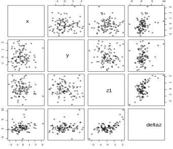
Figure 2illustrates one realization of the data generation with σ =1 in a pair plot. It can be seen from the figure that the distributions for x, y and 1

z are random (the upper left 3 by 3 plots). Furthermore, ∆z is linearly related to x as seen from the upper right plot. The second plot on the right-side illustrates the linear relationship between ∆z and y under fixed 1

z and the third plot on the right-side illustrates the cubic rela-tionship between ∆z and 1

z . For σ =2, 3, and 4 (data not shown in figure), the corresponding pair plots would have larger variations.

4.1.3. Simulation Analysis

Four data sets for the four scenarios (e.g., σ =1, 2, 3, and 4) are simulated first. The simulated data are then fitted with Guastello’s cusp regression model using least squares method. The summary statistics of the analyses are given in Table 1. It can be seen from the table that for the Scenario where σ =1, all the parameters of the polynomial regression model are statistically highly significant

(

p<0.001

)

with 2

0.763

R = , indicating ade-quate data-cusp model fitting and F-statistic = 60.71 indicating highly significance of the polynomial regression model. The estimated ˆσ =1.053, slightly greater than the true σ =1. Since β₁, β₃ and β₄ are all highly significant, we conclude that the Guastello’s polynomial regression method is sufficient to detect the specified cusp.

Results of other three scenarios inTable 1 indicate that as σ increases, the goodness of data-model fitting declines. In the scenario where σ =2, the 2

R drops to 0.454, F-statistic drops to 15.61 (still significant), and the estimated σ =2.107, close to the true σ =2. In this case, both β₁ and β₃ remain significant, indicating

Figure 2. Example of simulated data when σ =1 where the distributions of x y, z₁ are standard normal (the upper left 3 by 3 plots) and the relationships between ∆z to x (as li-near), to y (as linear) and to z₁ (as cubic).

x

-1 0 1 2 -5 0 5 10

-2

-1

0

1

2

3

-1

0

1

2

y

z1

-2

-1

0

1

2

-2 -1 0 1 2 3

-5

0

5

10

-2 -1 0 1 2

[image:6.595.127.470.386.681.2]

the existence of a cusp. With regard to Scenario 3 where σ =3, the 2

R further drops to 0.278 and F-statistic to 7.227. The estimated σ =3.160, again close to its true σ =3. In this case, only β₁ is highly significant and β₃ marginally significant, indicating that a cusp is likely. In Scenario 4 where σ =4, none of the esti-mated parameters required to support the cusp is statistically significant. Therefore, we could not be able to de-termine if the data contain a cusp. A power analysis is needed to assess if the sample size

(

n=100

)

is ade-quate.

4.1.4. Sample Size Estimation

To demonstrate the proposed novel simulation method, we estimate sample sizes needed for each of the four scenarios to achieve 85% statistical power employing this method and the estimated parameter

(

0, 1, 2, 3, 4, 5

)

β = β β β β β β and the estimated

σ

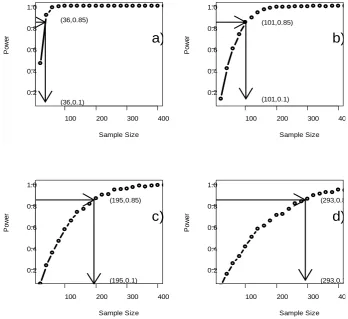
from Table 1 in the previous step. Figure 3summarizes the results. Data in Figure 3 indicate that with 85% statistical power to detect the underlying cusp, the required sample sizes for Scenarios 1 through 4 are 36, 101, 195 and 293, respectively. The required sample size varies proportionately with measurement errors. This result adds more evidence supporting the validity of the simula-tion-based approach we proposed for power analysis.

4.1.5. Reverse-Verification

[image:7.595.124.473.364.683.2]

If the novel simulation-based approach is valid, the sample size estimates for each of the four scenarios de-scribed in previous section will allow approximately 85% chance to detect the underlying cusp. Therefore, we took a reverse approach to compute statistical power by applying the calculated sample size as input for each of the four scenarios. Results in Figure 3 indicated that for Scenario 1, a sample size of 36 observations will be adequate to detect the cusp with 85% statistical power.

Figure 3. Statistical power curves corresponding to σ =1 in plot a), σ =2 in plot b), 3

σ = in plot c) and σ =4 in plot d). The arrows illustrate the sample size determination

from power of 0.85 to calculate the sample size required. 100 200 300 400

0.2 0.4 0.6 0.8 1.0 Sample Size P ow er (36,0.85) (36,0.1)

a)

100 200 300 40 0.2 0.4 0.6 0.8 1.0 Sample Size P ow er (101,0.85) (101,0.1)

b)

100 200 300 400 0.2 0.4 0.6 0.8 1.0 Sample Size P ow er (195,0.85) (195,0.1)

c)

[image:8.595.103.496.111.300.2]

Table 1. Parameter estimates, 2

R , Estimated σ2 _{and F-Statistic from four simulations with} σ =_{1, 2, 3}

and 4. The rows bolded are corresponding to the cusp determination.

1

σ= σ=2 σ=3 σ=4

0

β (Intercept) 0.487*** _{0.473. 0.459 0.446}

( )

3 1 z1

β 0.540*** _0.581*** _0.621*** _0.661***

( )

2 2 z1

β 0.456*** _0.411* _{0.367 0.323}

( )

3 y z1

β ∗

0.360** _{0.221 0.081 −0.058}

( )

4 x

β 0.563*** 0.626** 0.689* 0.753

( )

5 y

β 0.468*** _{0.435. 0.403 0.371}

2

R 0.763 0.454 0.278 0.1856

Estimated σ2 _{1.053 2.107 3.160 4.214}

F-Statistic with df = (5, 94) 60.71*** _15.61*** _7.227*** _4.286*

Significant codes: *** _{p-value < 0.00001,} **_{p-value < 0.001,} *_{p-value < 0.01, “.”(p-value < 0.05).}

To demonstrate this result, we make use Monte-Carlo procedure and randomly sample 36 observations from the simulate data

(

n=100

)

used for Scenario 1

(

σ =1

)

. We then fit the data to the Guastello’s cusp regres-sion model. We use the same criteria (significant β₁, plus either β₃ or β₄) to assess the detection of a cusp. Among 1000 repeats of the Monte-Carlo simulations with sample size n=36, we found 833 times (83.3%) significant. This result indicates that the power analysis of the simulation method we proposed is close to 85%. In another word, the method we proposed is slightly conservative, which is good for research design. The tem-plate is designed so that author affiliations are not repeated each time for multiple authors of the same affiliation. Please keep your affiliations as succinct as possible (for example, do NOT post your job titles, positions, aca-demic degrees, zip codes, names of building/street/district/province/state, etc.). This template was designed for two affiliations.

4.2. Verification with Published Data

The best approach to demonstrate the validity of the simulation approach would be to test it with observed data. To use our approach, we need two sets of data from any reported study: parameter estimates as effect size

(

0, 1, 2, 3, 4, 5

)

β = β β β β β β and estimated mean error of model fitting ˆσ . However, we experienced difficulties in finding such data from all the studies we accessed in the published literature database. For example, all β coefficients were reported by all studies but β₀ was not; furthermore, data-model fitting error fitting ˆσ was never reported in any of the published studies using Guastelle’s cusp polynomial regression method. Fortunately, one author of this paper [12] published a study that modeled early sexual initiation among young adolescents using this polynomial regression approach.

To verify the simulation-based method, the parameter effect size estimates were obtained from the paper with

(

0, 1, 2, 3, 4, 5

)

c

(

0.0309, 0.0726, 0.4819, 0.1236, 0.0613, 0.2693

)

β = β β β β β β = − − − − , and the data-model fitting

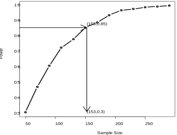
error σ =ˆ 0.5033 was obtained by accessing to the original computing records. With these estimates, the simu-lation-based approach in Section 3.2 is applied. Figure 4 presents the sample size-power curve. From the figure it can be seen that the estimated sample size is 153 to achieve 85% power. This sample size is much smaller than the sample

(

n=469

)

in the original study.

5. Discussions

In the case where analytical solution to power analysis and sample size determination is difficult, simulation represents an ideal alternative as recommended in [16] [17] [24]. In this paper, we reported a novel simulation- based approach we developed to estimate the statistical power and to compute sample size for Gustello’s poly-nomial cusp catastrophe model. The method was developed based on statistical power theory and our under-standing of Guastello’s cusp polynomial regression modeling approach. The computing method is programmed using the R software. Results from 1000 repeats of Monte Carlo simulation and empirical data analysis sug-gest that the method we proposed is valid and can be used in practice to conduct power analysis and to estimate sample size for Guastello polynomial cusp modeling method.

With this approach, researchers can compute statistical power and estimate sample size if they plan to conduct cusp modeling analysis using Gustallo’s polynomial regression method. A detailed introduction to the method can be found in [6] [7] [21]. Data needed for our methods included parameter effect size estimates for the inter-cept and five model parameters

(

β β β β β β₀, ₁, ₂, ₃, ₄, ₅

)

and a data-model fitting error σ or its estimate. With the specification of these data, power can be computed for any given sample sizes. In addition to computer power, the commonly used sample size-power curve can be generated to provide a visual presentation between sample size and statistical power. With such power curve, sample size can be estimated for specified power in design and analysis data from cusp catastrophe model.

[image:9.595.126.474.438.704.2]

To make the presentation easier, we confined this novel simulation approach to the situation of one regressor for each control variable in the cusp model. This approach can be easily adopted and extended to multiple re-gressors for each of the asymmetric

( )

x and bifurcation

( )

y variables where the Guastello’s cusp polynomial regression model would need to be extended.

Figure 4.Power curve for Chen et al. (2010). The estimated sample size for power of 0.85 is 153.

50 100 150 200 250

0.3 0.4 0.5 0.6 0.7 0.8 0.9 1.0

Sample Size

P

ow

er

(153,0.85)

More and more data suggest the utility of cusp modeling approach in characterizing a number of human be-haviors, particularly health risk bebe-haviors, such as tobacco smoking, alcohol consumption, hardcore drug use, dating violence, and unprotected sex [10] [11] [14] [21] [25] [26]. The methods we reported in this paper pro-vide a useful tool for researchers to more effectively design their research to investigate these risk behaviors and to assess intervention programs for risk reduction.

By conducting this study, we also note that previous studies published in the literature do not report adequate information for power analysis. We highly recommend that journal editors ask authors to report all parameter estimates, including β₀, and data-model fitting error (mean square of error). In addition to power analysis and sample size estimation, such data are also useful for readers to statistically assess appropriateness of the reported results.

There are a number of strengths with the method we present in this study. The principle and the computing process are not difficult to follow; the data used for the computing can be obtained; the computing software is written with R, available from the authors by request for collaboration; and the computing does not require much time (several seconds to half minutes). We are encouraged on the results from this research and work on extending the results into stochastic catastrophe model in [4] [19]. Despite many advantages, further application of the method in practice is needed.

Acknowledgements

This research was support in part by two NIH grants, one from the National Institute On Drug Abuse (NIDA, R01 DA022730, PI: Chen X) and another from the Eunice Kennedy Shriver National Institute of Child Health and Human Development (NICHD, R01HD075635, PIs: Chen X and Chen D).

References

[1] Thom, R. (1975) Structural Stability and Morphogenesis. Benjamin-Addison-Wesley, New York.

[2] Thom, R. and Fowler, D.H. (1975) Structural Stability and Morphogenesis: An Outline of a General Theory of Models. W. A. Benjamin, Michigan.

[3] Cobb, L. and Ragade, R.K. (1978) Applications of Catastrophe Theory in the Behavioral and Life Sciences. Behavioral Science, 23, 291-419. http://dx.doi.org/10.1002/bs.3830230511

[4] Cobb, L. and Watson, B. (1980) Statistical Catastrophe Theory: An Overview. Mathematical Modelling, 1, 311-317.

http://dx.doi.org/10.1016/0270-0255(80)90041-X

[5] Cobb, L. and Zacks, S. (1985) Applications of Catastrophe Theory for Statistical Modeling in the Biosciences. Journal of the American Statistical Association, 80, 793-802. http://dx.doi.org/10.1080/01621459.1985.10478184

[6] Guastello, S.J. (1982). Moderator Regression and the Cusp Catastrophe: Application of Two-Stage Personnel Selection, Training, Therapy and Program Evaluation. Behavioral Science, 27, 259-272. http://dx.doi.org/10.1002/bs.3830270305

[7] Guastello, S.J. (1989) Catastrophe Modeling of the Accident Processes: Evaluation of an Accident Reduction Program Using the Occupational Hazards Survey. Accident Analysis and Prevention, 21, 61-77.

http://dx.doi.org/10.1016/0001-4575(89)90049-3

[8] Grasman, R.P., van der Mass, H.L. and Wagenmakers, E. (2009) Fitting the Cusp Catastrophe in R: A Cusp Package Primer. Journal of Statistical Software, 32, 1-27.

[9] Clair, S. (1998) A Cusp Catastrophe Model for Adolescent Alcohol Use: An Empirical Test. Nonlinear Dynamics,

Psychology, and Life Sciences, 2, 217-241. http://dx.doi.org/10.1023/A:1022376002167

[10] Mazanov, J. and Byrne, D.G. (2006) A Cusp Catastrophe Model Analysis of Changes in Adolescent Substance Use: Assessment of Behavioural Intention as a Bifurcation Variable. Nonlinear Dynamics, Psychology, and Life Sciences,

10, 445-470.

[11] Guastello, S.J., Aruka, Y., Doyle, M. and Smerz, K.E. (2008) Cross-Cultural Generalizability of a Cusp Catastrophe Model for Binge Drinking among College Students. Nonlinear Dynamics, Psychology and Life Sciences, 12, 397-407.

[12] Chen, X., Lunn, S., Harris, C., Li, X., Deveaux, L., Marshall, S., et al. (2010) Modeling Early Sexual Initiation among Young Adolescents Using Quantum and Continuous Behavior Change Methods: Implications for HIV Prevention.

Nonlinear Dynamics, Psychology and Life Sciences, 14, 491-509.

[13] Wagner, C.M. (2010) Predicting Nursing Turnover with Catastrophe Theory. Journal of Advanced Nursing, 66, 2071- 2084.

Controlled Trial of an Adolescent HIV Prevention Program among Bahamian Youth: Effect at 12 Months Post-Interven- tion. AIDS and Behavior, 13, 495-508.

[15] Cohen, J. (1988) Statistical Power Analysis for the Behavioral Sciences. 2nd Edition, Lawrence Berbaum Associates, Hillsdale.

[16] Chow, S., Shao, J. and Wang, H. (2008) Sample Size Calculations in Clinical Research. 2nd Edition, Chapman and Hall/CRC, Boca Raton.

[17] Chen, D.G. and Peace, K.E. (2011) Clinical Trial Data Analysis Using R. Chapman and Hall/CRC, Boca Raton.

[18] Saunders, P.T. (1980) An Introduction to Catastrophe Theory. Cambridge University Press, Cambridge.

http://dx.doi.org/10.1017/CBO9781139171533

[19] Hartelman, A.I. (1997) Stochastic Catastrophe Theory. University of Amsterdam, Amsterdam.

[20] Iacus, S.M. (2008) Simulation and Inference for Stochastic Differential Equations with R Examples. Springer, Berlin.

http://dx.doi.org/10.1007/978-0-387-75839-8

[21] Guastello, S.J. and Gregson, A.M. (2011) Nonlinear Dynamic Systems Analysis for the Behavioral Sciences Using Real Data. CPC Press, Boca Raton.

[22] Gong, J., Stanton, B., Lunn, S., Devearus, L., Li, X., Marshall, S., Brathwaite, N.V., Cottrell, L., Harris, C. and Chen, X. (2009) Effects through 24 Months of an HIV/AIDS Prevention Intervention Program Based on Protection Motiva-tion Theory among Preadolescents in the Bahamas. Pediatrics, 123, 917-928.

http://dx.doi.org/10.1542/peds.2008-2363

[23] Chen, X., Stanton, S., Chen, D.G. and Li, X. (2013) Is Intention to Use Condom a Linear Process? Cusp Modeling and Evaluation of an HIV Prevention Intervention Trial. Nonlinear Dynamics, Psychology and Life Sciences, 17, 385-403.

[24] Bolker, B. (2008) Ecological Models and Data in R. Princeton University Press, Princeton.

[25] Mazanov, J. and Byrne, D.G. (2008) Modeling Change in Adolescent Smoking Behavior: Stability of Predictors across Analytic Models. British Journal of Health Psychology, 13, 361-379. http://dx.doi.org/10.1348/135910707X202490