Continued Fraction Method for Approximation of Heat Conduction Dynamics in a Semi Infinite Slab

(1)

http://dx.doi.org/10.4236/am.2014.57100

Continued Fraction Method for

Approximation of Heat Conduction

Dynamics in a Semi-Infinite Slab

Jietae Lee, Dong Hyun Kim

Department of Chemical Engineering, Kyungpook National University, Taegu, South Korea Email: [email protected], [email protected]

This work is licensed under the Creative Commons Attribution International License (CC BY). http://creativecommons.org/licenses/by/4.0/

Abstract

Heat conduction dynamics are described by partial differential equations. Their approximations with a set of finite number of ordinary differential equations are often required for simpler com-putations and analyses. Rational approximations of the Laplace solutions such as the Pade ap-proximation can be used for this purpose. For some heat conduction problems appearing in a semi-infinite slab, however, such rational approximations are not easy to obtain because the Lap-lace solutions are not analytic at the origin. In this article, a continued fraction method has been proposed to obtain rational approximations of such heat conduction dynamics in a semi-infinite slab.

Keywords

Heat Conduction Dynamics, Semi-Infinite Slab, Continued Fraction, Pade Approximation

1. Introduction

(2)

Consider the heat equation

2

2, 0 , 0

T T

x L t

t x

∂ ₌∂ _{< <} _<

∂ ∂ (1)

subject to

( )

, 0 0,

( )

0,

( )

,

( )

, 0

T x = T t = f t T L t = (2) Here x is the one-dimensional space variable, t is the normalized time variable and T(x,t) is the temperature that is varying by f(t) at x = 0 and fixed to 0 at x = L. Applying the Laplace transformation for the variable t, we have [8]

( )

, sinh

(

_{( )}

)

( )

sinh

L x s

T x s F s

L s −

= (3)

Here

( )

( ) ( )

0

, exp , d

T x s ≡

∫

∞ −s

τ

T x

τ τ

and

( )

( ) ( )

0exp d

F s ≡

∫

∞ −s

τ

f

τ τ

. As L goes to infinity, Equation (3) becomes

( )

, exp

(

)

( )

,

T x s = −x s F s L→ ∞ (4)

Equation (4) is the Laplace domain solution of the heat equation in a semi-infinite slab. G s

( )

=exp

( )

− s is the transfer function relating the forcing function F(s) and the temperature T(1,s). By scaling s, it can be used for x other than 1.

When the transfer function G(s) is approximated by a rational transfer function as

( )

_{( )}

1 1 2 2

1 2

n n

n

n n n

n

B s b s b s b

G s

A s s a s a s a

− − − − + + + ≈ = + + + + 

 (5)

the partial differential Equation (1) with the initial and boundary conditions of Equation (2) can be replaced by a set of ordinary differential equation [9] which is easy to solve for any arbitrary forcing function of f(t),

( )

( ) (

) ( )

1 2 1

1

1 0 0 0 0

0 1 0 0 0

0 0 1 0 0

1,

n n

a a a a

z t z t f t

T t b b b b z t

− − − − − −                 = +                 =            (6)

For the approximation of Equation (5), the Pade approximation method is often used, but it cannot be applied to our transfer function of G s

( )

=exp

(

−x s

)

unfortunately because the transfer function is not analytic at the origin. Here a method to overcome this difficulty is investigated.

2. Continued Fraction Expressions of

exp

( )

−

s

Rational approximation of exp

( )

− s is considered. Among two values of the square root of a complex s, only the root in right half complex plane is physically meaningful and used here. Since the series expansion and the continued fraction expansion in s do not exist at the origin, we consider a continued fraction expansion in the hyperbolic cosine function. From

( )

_{( )}

1

_{( )}

1

_{( )}

exp

exp 2 cosh exp

s

s s s

− = =

− − (7)

(3)

( )

_{( )}

( )

1 exp 1 2 cosh 1 2 cosh 2 cosh

1 1 1

2 cosh 2 cosh 2 cosh

s

s s s

− = − − − ≡ − − −   (8)

Equation (8) converges for s such that [5]

( )

2 cosh s ≥2 (9) The convergence condition of Equation (9) includes the right half complex plane of s which is important for the approximation of transfer function G(s) [10].

The right hand side of Equation (8), when truncated, is analytic and the series expansion in s exists. With 75

( )

cosh s terms in Equation (8), we can obtain a continued fraction expansion in s as

( )

0

1 2

0.98718 25.833 387.52 exp

1 1 1

1 1

1

h s s

s h s h s − = = + + + + + +   (10)

Here hi’s are given in Table 1. Truncating Equation (10) and rearranging, approximate rational transfer func-tions in the form of Equation (5) can be obtained and given in Table 2. For this, Maple routines such as ‘cfrac’ and ‘convert’ are used [7].

Equation (8) converges rather slowly near s = 0. To speed-up the convergence, the following continued frac-tion may be used.

( )

(

)

( )

(

)

(

)

( )

(

)

2 2 2 1 exp

2 cosh exp

1 1 2 cosh

2 cosh exp

1 2 cosh 1 2 cosh

s s s s s s s s α α α α α α α α α α α α − = − − = − − − = − − (11)

However, its conversion to the form of Equation (10) is difficult (our computer fails to the task for α = 2 due to the memory size problem).

3. Simulations

There are several methods to convert partial differential equations to ordinary differential equations [11]. Each method has its own merits and demerits, and direct comparisons are difficult. Here the simplest finite difference method (FDM) is used to illustrate the performance of the proposed method. The FDM method can be applied to the slab with a finite length (L) and the approximation of [8] [11]

(

)

(

)

(

)

(

)

2

2 2

1 , 2 , 1 ,

x k x

T k x t T k x t T k x t

T

x _{= ∆} x

+ ∆ − ∆ + − ∆

∂ _≈

∂ ∆ (12)

Case 1: Responses for a step forcing, f(t) = 1, are compared. Since F(s) = 1/s, Equation (4) for x = 1 becomes

( )

1, exp

( )

exp

( )

T s = − s F s = − s s and its analytic inversion is [8]

( )

1, erfc 0.5

(

)

(4)

Table 1.Constants in Equation (10).

h0 h1 h2 h3 h4 h5 h6

0.9871795 25.833333 387.516667 177.223806 89.759543 64.329228 38.382429

h7 h8 h9 h10 h11 h12 h13

33.586195 20.810544 20.918549 12.772382 14.518649 8.406289 10.907154

h14 h15 h16 h17 h18 h19

[image:4.595.85.540.200.488.2]

5.708357 8.808881 3.794178 7.840209 2.055945 9.060914

Table 2.Approximate rational transfer functions.

Order Approximate Rational Transfer Function

1 7.69231E 2 0.9871795

3.87097E 2 1 25.83333

s s

− ₌

+ − +

2 5.29764E 5 1.21718E 1

1.71610E 3 1.27279E 1

s s

− ₊ −

+ − + −

3 4.17239E 5 3.96591E 4 2.37921E 1

1.62304E 3 8.01919E 3 2.60873E 1

s s s

− ₊ − ₊ −

+ − + − + −

4 4.15846E 5 1.79084E 4 1.72118E 3 3.69655E 1

1.62222E 3 6.56117E 3 2.19943E 2 4.31843E 1

s s s s

− ₊ − ₊ − ₊ −

+ − + − + − + −

5 4.15842E 5 1.66537E 4 5.04522E 4 5.30220E 3 4.98132E 1

1.62222E 3 6.49028E 3 1.53275E 2 4.75865E 2 6.29315E 1

s s s s s

− ₊ − ₊ − ₊ − ₊ −

+ − + − + − + − + −

6 4.15842E 5 1.66205E 4 3.83649E 4 1.25068E 3 1.271830E 2 6.06194E 1

1.62222E 3 6.48890E 3 1.46426E 2 2.91596E 2 8.83094E 2 8.38651E 1

s s s s s s

− ₊ − ₊ − ₊ − ₊ − ₊ −

+ − + − + − + − + − + −

8

4.15842E 5 1.66202E 4 3.73453E 4 6.68900E 4 1.62222E 3 6.48889E 3 1.46000E 2 2.59761E 2 1.37727E 3 5.34402E 3 4.11291E 2 7.19763E 1

4.21218E 2 7.82521E 2 2.17456E 1 1.21075

s s s s

− ₊ − ₊ − ₊ −

+ − + − + − + −

− − − −

+ + + +

+ − + − + − +

10

4.15842E 5 1.66202E 4 3.73449E 4 6.62648E 4 1.03240E 3 1.62222E 3 6.48889E 3 1.46000E 2 2.59556E 2 4.05540E 2 1.51632E 3 3.10510E 3 1.06167E 2 5.97219E 2

5.84561E 2 8.36398E 2 1.40357E 1 3.24

s s s s s

s s s s

− ₊ − ₊ − ₊ − ₊ −

+ − + − + − + − + −

− − − −

+ + + +

+ − + − + − +

7.26206E 1 676E 1 s 1.35305

− +

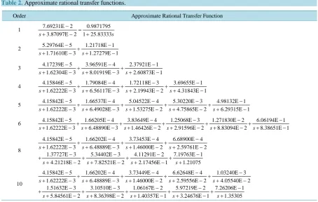
Ordinary differential equations of Equation (6) based on approximate rational transfer functions in Table 2 are solved for f(t) = 1. Responses are compared in Figure 1. The proposed method with n = 5 and the FDM me-thod with L = 6 and Δx = 1 have the same number of ordinary differential equations. The FDM method shows a large offset at a large time. To make the offset be less than the proposed method, L should be more than 78 and, correspondingly, the number of ordinary differential equations should be more than 77.

Case 2: Responses for a forcing,

( )

e erfct

( )

f t = t , are compared. Its Laplace transform is [8]

( )

1

(

1

)

F s = s s+ (14)

Equation (4) for x=1 becomes T

( )

1,s =exp

( )

− s F s

( )

=exp

( )

− s

(

s

(

s+1

)

and its analytic inversion is [8]

( )

1

(

)

1, et erfc 0.5

T t = + t+ t (15)

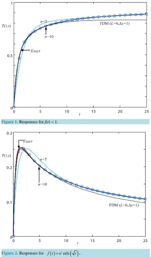
Responses of our approximations in Table 2 and the FDM method with L = 6 and Δx = 1 are shown in Figure 2. Similar conclusions as the above case can be drawn.

4. Conclusion

(5)

[image:5.595.158.470.85.615.2]

Figure 1.Responses for f(t) = 1.

Figure 2.Responses for

( )

e erfct

( )

f t = t .

tial equation) in the semi-infinite slab by the Laplace transformation method is proposed. The truncated contin-ued fraction can be used to convert the partial differential equation to a set of ordinary differential equations, making simulations and analyses simple.

Acknowledgements

(6)

References

[1] Carslaw, H.S. and Jaeger, J.C. (1989) Conduction of Heat in Solids. Oxford University Press, Oxford.

[2] Lee, J. and Kim, D.H. (1998) High-Order Approximations for Noncyclic and Cyclic Adsorption in a Particle. Chemical Engineering Science, 53, 1209-1221. http://dx.doi.org/10.1016/S0009-2509(97)00412-0

[3] Kim, D.H. and Lee, J. (1999) High-Order Approximations for Noncyclic and Cyclic Adsorption in a Biporous Adsor- bent. Korean Journal of Chemical Engineering, 16, 69-74. http://dx.doi.org/10.1007/BF02699007

[4] Lee, J. and Kim, D.H. (2011) Simple High-Order Approximations for Unsteady-state Diffusion, Adsorption and Reac- tion in a Catalyst: A Unified Method by a Continued Fraction for Slab, Cylinder and Sphere Geometries. Chemical Engineering Journal, 173, 644-650. http://dx.doi.org/10.1016/j.cej.2011.08.029

[5] Lorentzen, L. and Waadeland, H. (1992) Continued Fractions with Applications. Nort-Holland, New York.

[6] Chen, C.F. and Shieh, L.S. (1969) Continued Fraction Inversion by Routh’s Algorithm. IEEE Transactions on Circuit Theory, 16, 197-202. http://dx.doi.org/10.1109/TCT.1969.1082925

[7] (2012) Maple, Waterloo Maple Software Inc. www.maplesoft.com

[8] Zill, D.G. and Cullen, M.R. (1992) Advanced Engineering Mathematics. PWS-KENT Pub., Boston. [9] Kailath, T. (1980) Linear Systems. Prentice-Hall, New Jersey.