www.hydrol-earth-syst-sci.net/19/857/2015/ doi:10.5194/hess-19-857-2015
© Author(s) 2015. CC Attribution 3.0 License.
Calibration approaches for distributed hydrologic models
in poorly gaged basins: implication for streamflow
projections under climate change
S. Wi1, Y. C. E. Yang1, S. Steinschneider1, A. Khalil2, and C. M. Brown1
1Department of Civil and Environmental Engineering, University of Massachusetts Amherst, USA 2The World Bank, Washington, DC, USA
Correspondence to: S. Wi ([email protected])
Received: 10 August 2014 – Published in Hydrol. Earth Syst. Sci. Discuss.: 17 September 2014 Revised: 13 January 2015 – Accepted: 20 January 2015 – Published: 10 February 2015
Abstract. This study tests the performance and uncertainty of calibration strategies for a spatially distributed hydrologic model in order to improve model simulation accuracy and understand prediction uncertainty at interior ungaged sites of a sparsely gaged watershed. The study is conducted using a distributed version of the HYMOD hydrologic model (HY-MOD_DS) applied to the Kabul River basin. Several cali-bration experiments are conducted to understand the bene-fits and costs associated with different calibration choices, including (1) whether multisite gaged data should be used simultaneously or in a stepwise manner during model fit-ting, (2) the effects of increasing parameter complexity, and (3) the potential to estimate interior watershed flows using only gaged data at the basin outlet. The implications of the different calibration strategies are considered in the context of hydrologic projections under climate change. To address the research questions, high-performance computing is uti-lized to manage the computational burden that results from high-dimensional optimization problems. Several interesting results emerge from the study. The simultaneous use of mul-tisite data is shown to improve the calibration over a step-wise approach, and both multisite approaches far exceed a calibration based on only the basin outlet. The basin out-let calibration can lead to projections of mid-21st century streamflow that deviate substantially from projections under multisite calibration strategies, supporting the use of caution when using distributed models in data-scarce regions for cli-mate change impact assessments. Surprisingly, increased pa-rameter complexity does not substantially increase the un-certainty in streamflow projections, even though parameter
equifinality does emerge. The results suggest that increased (excessive) parameter complexity does not always lead to in-creased predictive uncertainty if structural uncertainties are present. The largest uncertainty in future streamflow results from variations in projected climate between climate models, which substantially outweighs the calibration uncertainty.
1 Introduction
hydrolog-ical response at interior ungaged sites, a benefit not afforded by lumped models. The use of distributed hydrologic mod-eling for interior point streamflow estimation is particularly relevant for poorly gaged river basins in developing coun-tries, where reliable predictions at interior sites are often required to inform water infrastructure investments. As in-ternational development agencies begin to integrate climate change considerations into their decision-making processes (e.g., Yu et al., 2013), these investments need to be robust under both current climate conditions and possible future cli-mate regimes.
Despite their roots in physical realism, distributed hydro-logic models can suffer from substantial uncertainty. A major source of uncertainty originates from the proper identifica-tion of parameter values that vary across the watershed, espe-cially when observed streamflow data is only available at one or a few points (Exbrayat et al., 2014). Parameters can be dis-cretized across the watershed in several ways (Flugel, 1995; Efstratiadis et al., 2008; Khakbaz et al., 2012): uniquely for each grid cell or hydrologic response unit (fully distributed), based on sub-basins whose boundaries do not necessarily ensure homogenous characteristics (semi-distributed) or, in the simplest case, a single parameter set for all model grid cells (lumped). With limited data, the parameter identifica-tion problem, particularly for the fully distributed case, can be impractical or infeasible (Beven, 2001). The parameteri-zation challenge has spurred substantial advances in under-standing appropriate calibration techniques for distributed hydrologic models. Many studies have attempted to reduce the dimensionality of the calibration problem to alleviate the issue of equifinality (Beven and Freer, 2001), which is the phenomenon whereby multiple parameter sets produce in-distinguishable model performance. This work has found fa-vorable results when the parametric complexity of the dis-tributed model is aligned with the data available for calibra-tion (Leavesley et al., 2003; Ajami et al., 2004; Eckhardt et al., 2005; Frances et al., 2007; Zhu and Lettenmaier, 2007; Cole and Moore, 2008; Pokhrel and Gupta, 2010; Khakbaz et al., 2012). There has also been extensive research exploring the use of multiple objectives and different operational proce-dures to understand parameter estimation tradeoffs and iden-tifiability for distributed model calibration, with great suc-cess (Madsen, 2003; Efstratiadis and Koutsoyiannis, 2010; Li et al., 2010; Kumar et al., 2013).
Despite these advances, important questions still persist. It still remains difficult to compare the uncertainty that emerges from different operational calibration procedures for mul-tisite applications (i.e., whether gages in series should be used sequentially or simultaneously for calibration) and un-der different levels of parametric complexity. Due to the computational burden required to calibrate distributed mod-els, this uncertainty is problematic to explore. Furthermore, in poorly gaged basins, it is challenging to quantify the lost accuracy and increased uncertainty for interior flow estima-tion when a distributed model is calibrated only at an
out-let gage (which is often all that is available in developing-country river basins). In the case of significant spatial vari-ability in the basin properties that influence runoff generation (e.g., permeability, vegetation, and slope), accurate runoff predictions are unlikely at interior locations based only on the lumped information obtained at the basin outlet (Ander-son et al., 2001; Cao et al., 2006; Breuer et al., 2009; Lerat et al., 2012; Smith et al., 2012; Wang et al., 2012). The extent of this error and uncertainty is not well understood for het-erogeneous basins due to the computational expense required to explore this issue. Finally, rarely have the implications of these calibration issues been explicitly examined for possi-ble future climate conditions, which is required in climate change impact studies. This question has been explored for lumped, conceptual models (Wilby, 2005; Steinschneider et al., 2012), but has been difficult to evaluate for computation-ally expensive distributed models.
This study addresses the above research challenges by fo-cusing on the following four questions: (1) how does calibra-tion procedure for using multisite data affect the accuracy and uncertainty of distributed models used for streamflow predictions at ungaged sites; (2) what effects does increased parameter complexity have on distributed model calibration and prediction; (3) how much degradation in model accuracy and uncertainty can be expected for interior flow estimation based on a calibration procedure using only the basin out-let; and (4) how do different calibration formulations for a distributed model alter projections of streamflow at ungaged sites under climate change conditions? These questions are considered in an application of a distributed version of the daily HYMOD hydrologic model to the Kabul River basin in Afghanistan and Pakistan. To address these research ques-tions, high-performance computing is utilized to manage the computational burden that often hinders such explorations (Laloy and Vrugt, 2012; Zhang et al., 2013).
2 Study area
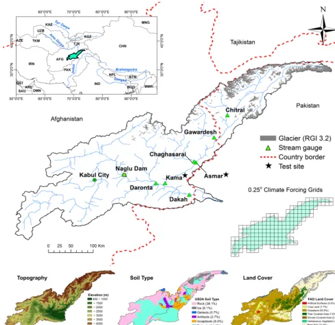
The Kabul River basin (67 370 km2) is a plateau sur-rounded by mountains located in the eastern central part of Afghanistan (Fig. 1). It is the most important river basin of Afghanistan, containing 35 % of the country’s population. While it encompasses just 12 % of the area of Afghanistan, the basin’s average annual streamflow (about 24 billion cu-bic meters) is about 26 % of the country’s total streamflow volume (World Bank, 2010).
Figure 1. Kabul River basin.
of Afghanistan has developed comprehensive plans for new hydropower projects on the Kabul River owing to its advanta-geous topography for the development of water storage and hydropower (IUCN, 2010), and recently reached an agree-ment with the Pakistan governagree-ment to work on a 1500 MW hydropower project on the Kunar River (one of major tribu-tary in the Kabul River basin) as part of the joint management of common rivers between the two countries (DAWN, 2013). The streamflow regime of the Kabul River can be classified as glacial with maximum streamflow in June or July and min-imum streamflow during the winter season. Approximately
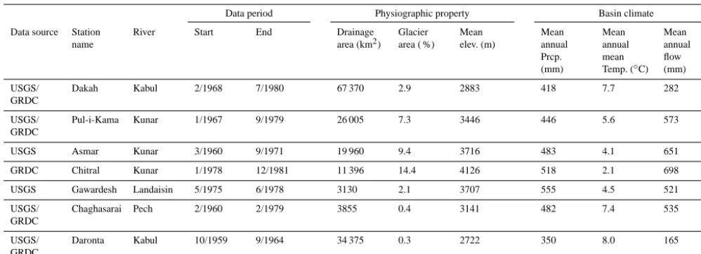
Table 1. Streamflow gaging stations in the Kabul River basin.
Data period Physiographic property Basin climate
Data source Station name
River Start End Drainage area (km2)
Glacier area ( %)
Mean elev. (m)
Mean annual Prcp. (mm)
Mean annual mean Temp. (◦C)
Mean annual flow (mm)
USGS/ GRDC
Dakah Kabul 2/1968 7/1980 67 370 2.9 2883 418 7.7 282
USGS/ GRDC
Pul-i-Kama Kunar 1/1967 9/1979 26 005 7.3 3446 446 5.6 573
USGS Asmar Kunar 3/1960 9/1971 19 960 9.4 3716 483 4.1 651
GRDC Chitral Kunar 1/1978 12/1981 11 396 14.4 4126 518 2.1 698
USGS Gawardesh Landaisin 5/1975 6/1978 3130 2.1 3707 555 4.5 521
USGS/ GRDC
Chaghasarai Pech 2/1960 2/1979 3855 0.4 3141 482 7.4 535
USGS/ GRDC
Daronta Kabul 10/1959 9/1964 34 375 0.3 2722 350 8.0 165
each sub-watershed delineated by the stations located inside the Kabul Basin (Fig. 1). Two different climate patterns are distinguishable across the sub-basins. The sub-basins on the Kunar River tributary (Kama, Asmar, Chitral, Gawardesh, and Chaghasarai) receive moderate annual precipitation and are highly affected by snow and glacier covers. All of these sub-basins have high ratios of mean annual flow to mean an-nual precipitation, with the ratios for the Kama, Asmar, Chi-tral, and Chaghasarai sub-basins larger than 1. Conversely, the Daronta sub-basin contains only minimal glacial cover, and is relatively dry. Daronta is also much less productive, with annual streamflow far below the other sub-basins with an average of only 165 mm yr−1.
Issues of shared water resources between Afghanistan and Pakistan in the Kabul River basin are becoming complex due to the impacts of climatic variability and change (IUCN, 2010). The vulnerability of glacial streamflow regimes to changes in temperature and precipitation (Stahl et al., 2008; Immerzeel et al., 2012; Radic et al., 2014) highlights the need to assess the impact of climate change on future water avail-ability in this area.
3 Data and models 3.1 Data
Gridded daily precipitation and temperature products with a spatial resolution of 0.25◦C were gathered between calendar
years 1961 and 2007 from the Asian Precipitation Highly Resolved Observational Data Integration Towards Evalua-tion (APHRODITE) data set (Yatagai et al., 2012). There has been some concern regarding underestimation of precipita-tion in APHRODITE for some regions of Asia (Palazzi et al., 2013); our preliminarily data analysis (intercomparison of precipitation products between five different databases) confirmed this for the Kabul River basin (shown in Fig. S1 in
the Supplement). Thus, the APHRODITE precipitation was bias-corrected by the precipitation product from the Univer-sity of Delaware global terrestrial precipitation (UD) data set (Legates and Willmott, 1990). Daily series of bias-corrected APHRODITE precipitation were coupled with APHRODITE temperature for 160 0.25◦C grid cells to produce a climate forcing data set for the distributed domain of the Kabul River basin model.
This study used the set of global climate change simula-tions from the World Climate Research Programme’s Cou-pled Model Intercomparison Project Phase 5 (CMIP5) mul-timodel ensemble (Talyor et al., 2012). Monthly climate outputs of GCMs (general circulation models) were down-scaled to a daily temporal resolution and 0.25◦C spatial res-olution based on the bias-correction spatial disaggregation (BCSD) statistical downscaling method introduced by Wood et al. (2004).
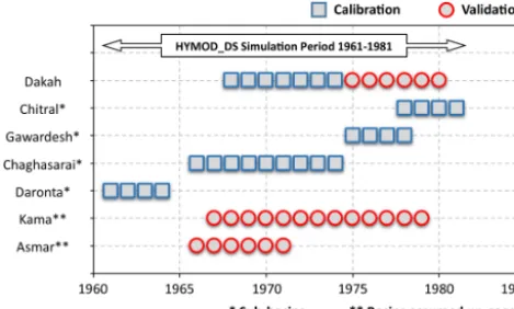
Figure 2. Streamflow data usage for the model calibration and
val-idation.
record at the Dakah station, located at the basin outlet, is also used for validation purposes.
The Randolph Glacier Inventory version 3.2 (RGI 3.2) data set (Pfeffer et al., 2014) was used to extract glacial cov-erage in the Kabul River basin, which totaled 5.7 % of the basin area (Fig. S2). In the hydrological modeling process, the model needs to be informed by reliable estimates on vol-ume of water retained in glaciers, especially for future sim-ulations under warming conditions. We followed the method proposed in Grinsted (2013), which uses multivariate scaling relationships to estimate glacier and ice cap volume based on elevation range and area. Specifically, the scaling law in-cluding area and elevation range factors was applied to esti-mate glacier/ice cap volume when the glacier depth exceeded 10 m. Otherwise, glacier/ice cap volume was estimated with the area–volume scaling law. The elevation range spanned by each individual glacier is estimated using the global dig-ital elevation model (DEM) from the shuttle radar topog-raphy mission (SRTMv4) in 250 m resolution (Jarvis et al., 2008). Density of ice (0.9167 g cm−3)is applied to calculate glacier/ice cap volume in meters of water equivalent.
The database for land covers and soil types of the Kabul River basin (Fig. 1) are provided by the Food and Agricul-ture Organization of the United Nations (Latham et al., 2014) and United States Department of Agriculture – Natural Re-sources Conservation Service Soils (USDA-NRCS, 2005), respectively.
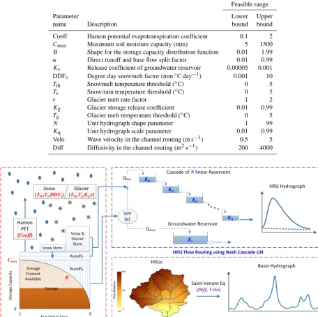
3.2 Distributed Hydrologic Model (HYMOD_DS) In this study the lumped conceptual hydrological model HY-MOD (Boyle, 2001) is coupled with a river routing model to be suitable for modeling a distributed watershed system. We name it HYMOD_DS denoting the distributed version of HYMOD. Snow and glacier modules have been introduced to enhance the modeling process for glacier and snow cov-ered areas within the Kabul River basin. The HYMOD_DS is composed of hydrological process modules that
repre-sent soil moisture accounting, evapotranspiration, snow pro-cesses, glacier processes and flow routing. The model op-erates on a daily time step and requires daily precipitation and mean temperature as input variables. The overall model structure of the HYMOD_DS and its 15 parameters are de-scribed in Fig. 3 and Table 2, respectively. Further details are provided below.
The HYMOD conceptual watershed model has been ex-tensively used in studies on streamflow forecasting and model calibration (Wagener et al., 2004; Vrugt et al., 2008; Kollat et al., 2012; Gharari et al., 2013; Remesan et al., 2013). The HYMOD is a soil moisture accounting model based on the probability–distributed storage capacity con-cept proposed by Moore (1985). This concon-ceptualization rep-resents a cumulative distribution of varying storage capaci-ties (C) with the following function:
F (C)=1−
1− C Cmax
B
0≤C≤Cmax, (1)
where the exponentBis a parameter controlling the degree of spatial variability of storage capacity over the basin and Cmaxis the maximum storage capacity. The model assumes that all storages within the basin are filled up to the same critical level (C∗(t )), unless this amount exceeds the storage capacity of that particular location. With this assumption, the total water storageS(t )contained in the basin corresponds to
S (t )= Cmax B+1 1−
1−C
∗
(t ) Cmax
B+1!
. (2)
Consequently, two parameters are introduced for the runoff generation process with two components:
Runoff1=
P (t )+C∗(t−1)−CmaxifP (t ) +C∗(t−1)≥Cmax
0 ifP (t )+C∗(t−1) < Cmax
, (3)
Runoff2=
(P (t )−Runoff1)+(S (t )−S (t−1)) ifP (t )−Runoff1≥S (t )−S (t−1) 0 ifP (t )−Runoff1< S (t )−S (t−1)
, (4)
whereP (t )is precipitation, Runoff1is surface runoff, and Runoff2is subsurface runoff. A parameter (α)is introduced to represent how much of the subsurface runoff is routed over the fast (Qfast)and slow (Qslow)pathway:
Qfast=Runoff1+α·Runoff2, (5)
Qslow=(1−α)·Runoff2. (6)
The potential evapotranspiration (PET) is derived based on the Hamon method (Hamon, 1961), in which daily PET in millimeters is computed as a function of daily mean temper-ature and hours of daylight:
PET=Coeff·29.8·Ld·
0.611·exp17.27· T (T+273.3)
Table 2. HYMOD_DS parameters.
Feasible range
Parameter Lower Upper
name Description bound bound
Coeff Hamon potential evapotranspiration coefficient 0.1 2
Cmax Maximum soil moisture capacity (mm) 5 1500
B Shape for the storage capacity distribution function 0.01 1.99
α Direct runoff and base flow split factor 0.01 0.99
Ks Release coefficient of groundwater reservoir 0.00005 0.001 DDFs Degree day snowmelt factor (mm◦C day−1) 0.001 10
Tth Snowmelt temperature threshold (◦C) 0 5
Ts Snow/rain temperature threshold (◦C) 0 5
r Glacier melt rate factor 1 2
Kg Glacier storage release coefficient 0.01 0.99
Tg Glacier melt temperature threshold (◦C) 0 5
N Unit hydrograph shape parameter 1 99
Kq Unit hydrograph scale parameter 0.01 0.99
Velo Wave velocity in the channel routing (m s−1) 0.5 5 Diff Diffusivity in the channel routing (m2s−1) 200 4000
Figure 3. Distributed version of the HYMOD model (HYMOD_DS).
whereLdis the daylight hours per day,T is the daily mean air temperature (◦C), and Coeff is a bias correction factor. The hours of daylight is calculated as a function of lati-tude and day of year based on the daylight length estimation model (CBM model) suggested by Forsythe et al. (1995).
The HYMOD_DS includes snow and glacier modules with separate runoff processes, i.e., the runoff from the glacierized area is calculated separately and added to runoff generated from the soil moisture accounting module cou-pled with the snow module. The implicit assumption here is that there is no interchange of water between soil layers and
glacial area and runoff from glacial areas is regarded as sur-face flow. The runoff from each area is weighted by its area fraction within the basin to obtain total runoff.
Ms=DDFs×(T−Ts) , (8) Mg=DDFg× T−Tg
, (9)
with DDFs (Ts)and DDFg(Tg)applied separately for snow and glacier modules, respectively. To account for the higher melting rate of glaciers than snow owing to the low albedo (Konz and Seibert, 2010; Kinouchi et al., 2013), we intro-duced a parameterr> 1 to constrain DDFgto be larger than DDFs (i.e., DDFg=r×DDFs). For the rain that falls on the glacierized area, the glacier parameterKgdetermines the portion of rain becoming surface runoff as a multiplier for the rainfall. The remaining rainfall is assumed to be accumulated to the glacier store.
The within-grid routing process for direct runoff is rep-resented by an instantaneous unit hydrograph (IUH) (Nash, 1957), in which a catchment is depicted as a series of N reservoirs each having a linear relationship between storage and outflow with the storage coefficient ofKq. Mathemati-cally, the IUH is expressed by a gamma probability distribu-tion:
u (t )= Kq 0 (N ) Kqt
N−1
exp −Kqt, (10)
where0is the gamma function. The within-grid groundwater routing process is simplified as a lumped linear reservoir with the storage recession coefficient ofKs.
The transport of water in the channel system is described using the diffusive wave approximation of the Saint-Venant equation (Lohmann et al., 1998):
∂Q ∂t +C
∂Q ∂x −D
∂2Q
∂2x2=0, (11)
whereCandDare parameters denoting wave velocity (Velo) and diffusivity (Diff), respectively.
Similar to most other hydrological models (Efstratisdis et al., 2008), HYMOD_DS is not designed to model water ab-stractions for agricultural lands and dam operations within the basin. According to the World Bank (2010), water de-mand for agricultural use is about 2000 million cubic me-ters, or about 8.3 % of the total annual flow. The Naglu dam (Fig. 1) upstream of the Daronta streamflow gage forms the largest and most important reservoir in the basin, with an ac-tive storage of 379 million cubic meters. In our hydrologic modeling process, the water consumed by irrigated crop-lands is implicitly accounted for by the evapotranspiration module. We note that the degree of irrigation impact dur-ing the time frame used for calibration (1960–1981) is likely much smaller than the current level. We also expect that using monthly data for calibration somewhat reduces the bias from human interference, particularly the daily operations of the Naglu dam. Nevertheless, the calibration results for the gage below this dam (Daronta), and to a lesser extent the basin
outlet (Dakah), should be approached with caution. Given that a majority of the gages examined in this study are on an underdeveloped branch of the Kabul River, issues of human interference on calibration are somewhat mitigated.
4 Methods
The purpose of this study is to explore the implications of different calibration strategies and choices for a compu-tationally expensive distributed hydrologic model. A vari-ety of calibration experiments are conducted, with the re-sults from preceding experiments informing choices made for subsequent ones. All calibration approaches are tested in terms of their ability to predict flows at interior site gages that were left out of the calibration process. In all cases, the genetic algorithm (GA) introduced by Wang (1991) is used as an optimization method for model parameter cali-bration, and the objective function is based simply on the Nash–Sutcliffe efficiency (NSE) (Nash and Sutcliff, 1970), which is by far the most utilized performance metric in hy-drological model applications (Biondi et al., 2012). A mul-tisite average of the NSE is used when evaluating perfor-mance across multiple sites. We fully recognize that the use of one objective, such as the NSE, is inferior compared to multiobjective approaches that can identify Pareto optimal solutions that provide good model performance across dif-ferent components of the flow regime (Madsen, 2003; Efs-tratiadis and Koutsoyiannis, 2010; Li et al., 2010; Kumar et al., 2013). However, in this particular study daily hydrologic model simulations can only be compared against available monthly streamflow records, reducing the number of viable objectives against which to calibrate. That is, statistics repre-senting peak flows, extreme low flows, and other daily flow regime characteristics often used in multiobjective optimiza-tion approaches are unavailable. We believe that the use of a monthly NSE value as a single objective, while coarse, does not inhibit our ability to provide insight into the research questions posed. In addition to the NSE, the Kling–Gupta efficiency (KGE) (Gupta et al., 2009) is adopted as an al-ternative model performance metric, which equally weights model mean bias, variance bias, and correlation with obser-vations.
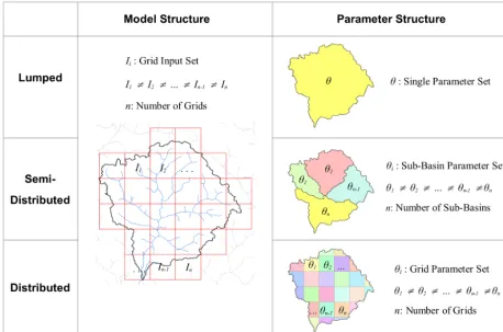
Figure 4. Model structure based on climate input grids and three different parameterization concepts.
structure follows the climate input grids; i.e., the hydrolog-ical water cycle within each grid cell is modeled separately. We note that a lumped model structure (i.e., no gridded or sub-unit structure) has often been considered as a baseline model formulation in the assessment of distributed model-ing frameworks (e.g., see Smith et al., 2013). However, the focus of our study is on ungaged interior site streamflow estimation, making this formation somewhat inappropriate. Furthermore, preliminary tests comparing streamflow sim-ulations at the basin outlet (Dakah) between a gridded and basin-averaged structure, both with a lumped parameter for-mulation, support the use of the distributed grid structure (Fig. S3).
The parameter complexity will vary depending on the cal-ibration experiment being conducted but, for each exper-iment regardless of the parameterization, the optimization is implemented 50 times using the GA algorithm to ex-plore calibration uncertainty. The considerably high compu-tational cost required to perform a large number of calibra-tions is managed using the parallel computing power pro-vided by the Massachusetts Green High-Performance Com-puting Center (MGHPCC), from which several thousands of processors are available.
In the first modeling experiment, we explore two calibra-tion strategies for using multisite streamflow data, a stepwise
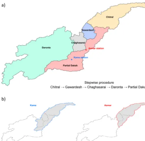
Figure 5. (a) Sub-basins corresponding to five gaging stations are
used for the multisite calibrations. (b) Two sub-basins (Kama and Asmar) are assumed to be ungaged and used for evaluating the cal-ibration approaches.
4.1 Multisite calibration: stepwise and pooled approaches
In the first experiment, the semi-distributed parameterization concept is compared under alternative multisite calibration strategies, the stepwise and pooled calibration approaches. To conduct the stepwise calibration, a nested class of sub-basins is defined corresponding to multiple gaging stations. In the first step of the stepwise calibration, the optimiza-tion process is carried out with nested sub-basins at the low-est level (i.e., the most upstream sites). Once parameters of nested sub-basins are determined, the parameters are fixed, and the calibration procedure proceeds with nested basins at upper levels until parameters for the entire basin are deter-mined. In this particular application to the Kabul River basin, five gaged sub-basins were selected and the stepwise calibra-tion procedure for those sub-basins followed this direccalibra-tion: Chitral→Gawardesh→Chaghasarai→Daronta→Dakah (Fig. 5). The stepwise calibration approach involves a num-ber of GA implementations corresponding to the numnum-ber of gaging sites. The GA optimization was carried out a total of 250 times in this application, with 50 optimization runs con-taining GA implementations for five sub-basin regions.
The pooled calibration strategy involves calibrating all pa-rameters of the model domain simultaneously against mul-tiple streamflow gages within the watershed. This approach aims at looking for suitable parameters that are able to pro-duce satisfactory model results at all gaging stations in a single implementation of GA optimization. That is, the GA
searches the entire parameter space at once to maximize the average NSE across all sites. This operational feature reduces the processing time spent on the GA implementation com-pared to the stepwise calibration strategy. To identify the bet-ter of the two multisite calibration approaches, the compar-ison focused on their ability to predict streamflow and cal-ibration uncertainties at two interior site gages (Kama and Asmar) that were assumed to be ungaged (Fig. 5), as well as for validation data at the basin outlet.
It is important to note that the evaluation of these multi-site calibration strategies is somewhat weakened because of the lack of overlapping data periods among most of the sta-tions (Fig. 2). This drawback prevents the calibration meth-ods from accounting for simultaneous information from dif-ferent tributaries, which, if available, would better enable the calibration methods to account for heterogeneity of hydro-logical processes across the sub-basins.
4.2 Increased parameter complexity
[image:9.612.50.284.67.296.2]4.3 Basin outlet calibration
The third experiment considers the situation where there is only gaged data at the basin outlet (Dakah) for calibration, a common situation when calibrating hydrologic models in data-scarce river basins. Here, we evaluate the potential of the basin outlet calibration to estimate interior watershed flows in terms of both accuracy and precision at all gaging stations. All levels of parameter complexity are considered for this calibration. The main purpose of this experiment is to compare the veracity of a distributed hydrologic model cali-brated only using basin outlet data with results from multisite calibrations to better understand the degradation in model performance under data scarcity. Other than the use of an NSE objective only at the basin outlet, all other GA settings for each level of parameter complexity are identical to the settings used in the second experiment.
4.4 Climate change projections of streamflow
The fourth experiment investigates how the choice of cali-bration approach can alter the projections of future flow under climate change. To explore this question, stream-flow simulations for the 2050s, defined as the 30-year period spanning from 2036 to 2065, are carried out using climate projections from the CMIP5 (Talyor et al., 2012). A total of 36 different climate models run under two future conditions of radiative forcing (RCP 4.5 and 8.5) are used. Streamflow projections are developed for the basin outlet (Dakah) and two interior gages left out of the calibration (Kama and As-mar). By using 36 different GCMs and 50 optimization trials for each calibration scheme, this analysis compares the un-certainty in future streamflow projections originating from uncertainty in different hydrologic model parameterization schemes and under alternative future climates.
Streamflow projections are considered under all three parameterization schemes (lumped, semi-distributed, and fully distributed) for both the basin outlet model and the best multisite calibration approach (stepwise or pooled). Multiple streamflow characteristics are evaluated, includ-ing monthly streamflow, wet (April–September) and dry (October–March) season flows, and daily peak flow re-sponse. The differences and uncertainty in these metrics across calibration approaches will highlight the importance of calibration strategy for evaluating future water availability and flood risk.
5 Results
For the remaining part of the paper, we introduce the following shorthand: Lump, Semi, and Dist indicate the lumped, semi-distributed, and fully distributed parameteriza-tion schemes, and Outlet, Stepwise, and Pooled correspond to basin outlet, stepwise, and pooled calibrations. The com-parison between different calibration strategies is based on
the model performance evaluated with the NSE, as well as an alternative metric, the KGE.
5.1 Pooled calibration vs. stepwise calibration
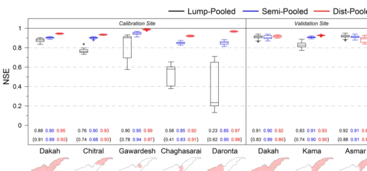
This section reports the results from the first experiment comparing the stepwise and pooled calibration approaches for the semi-distributed model parameterization. Figure 6 shows the comparison between the Stepwise and Semi-Pooled with box plots representing the 50 trials of calibra-tion. Under the stepwise calibration the results for four sub-basins (Chitral, Gawardesh, Chaghasarai, and Daronta) are optimal because there is no interaction between those basins. However, the calibrated parameter sets of each sub-basin act as constraints in the last step of the Semi-Stepwise resulting in the degradation of model skill at the basin out-let (Dakah) and two left-out gages (Asmar and Kama). This becomes apparent when comparing the Semi-Stepwise to the Semi-Pooled results. The model skill under the Semi-Pooled is similar to that from the Semi-Stepwise with respect to the four upstream sub-basins, but it outperforms at the verifi-cation gages. This is particularly true for the Asmar gage, which exhibits a downward bias and substantial variability in performance under the Semi-Stepwise. The Semi-Pooled results suggest that small sacrifices of model performance at certain sites can improve and stabilize basin-wide perfor-mance. Expected values of KGE from 50 calibrations are also provided (values in parenthesis in the bottom of Fig. 6) and this performance metric also leads to the same conclusion. Therefore, the Semi-Pooled was selected as the better multi-site calibration strategy and is considered for further analyses in the following sections.
5.2 Pooled calibration with alternative parameterizations
Figure 6. Comparison of the stepwise and pooled calibrations under the semi-distributed parameterization. Each calibration is conducted 50
times. Values on the bottom represent expected values of NSE (in upper row) and KGE (within parenthesis in lower row) from 50 calibrations.
Figure 7. Comparison of the pooled calibrations for the 3 parameterizations of lumped, semi-distributed, and distributed. Each calibration is
conducted 50 times. Values on the bottom represent expected values of NSE (in upper row) and KGE (within parenthesis in lower row) from 50 calibrations.
that the fully distributed conceptualization leads to overfit-ting of the model as compared to the Semi-Dist conceptu-alization. We reached the same conclusion when examining the KGE values, which rise with greater parameter complex-ity at calibration sites but no longer follow this pattern strictly at validation sites.
Interestingly, the Lump-Pooled performs well at the verifi-cation sites despite its poor performance at calibration sites. The Lump-Pooled does not show significant degradation in skill at Kama compared to the more complex parameteriza-tions, and the flow prediction at Asmar actually exhibits the best performance of all three model variants. A partial reason for this unexpected result arises from different overlapping periods in the calibration and validation data (see Fig. 2). The periods used for the calibration for Chitral (1978–1981) and Gawardesh (1975–1978) have no overlapping periods with
the one for Asmar (1966–1971), which encompasses those two sub-basins. Instead, the validation at Asmar is mostly affected by the calibration to Dakah because of the overlap-ping 4 years (1968–1971) between those two sites. This ex-plains the reason why the Lump-Pooled shows high skill at Asmar despite the low skill at its sub-basins. However, the low model skill at Chaghasarai from the Lump-Pooled propa-gates to the validation result at Kama, as these two sites have a relatively long overlapping period (8 years, from 1967 to 1974).
5.3 Limitations of the basin outlet calibration
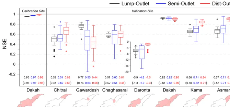
[image:11.612.114.484.285.457.2]Figure 8. Comparison of the basin outlet calibrations for the three parameterizations of lumped, semi-distributed, and distributed. Each
calibration is conducted 50 times. Values on the bottom represent expected values of NSE (in upper row) and KGE (within parenthesis in lower row) from 50 calibrations.
used for model validation. First, we consider the flows at Dakah. During the calibration period, all three parameteriza-tion schemes produce very accurate streamflow predicparameteriza-tions with NSE (KGE) values above 0.95 (0.96) (Fig. 8). High ac-curacy holds even under the Lump-Outlet, despite the spa-tial heterogeneity of the basin. While NSE and KGE values at Dakah rise marginally with greater parameter complexity during calibration, this no longer holds during the validation period, suggesting no benefit with an increase in parameter complexity.
The validation results for the six sub-basins demonstrate the danger in relying on outlet data alone when calibrating a distributed model for flow prediction at interior points. Streamflow predictions at interior sites exhibit low accu-racy and high uncertainty, with the worst performance at the Daronta site (all NSEs and KGEs are negative). We note that the poor performance at Daronta is likely due in part to the impacts of water abstraction and the operation of Naglu dam. Further examination (Fig. S4) showed that the HYMOD_DS significantly overestimated streamflow at Daronta and un-derestimated flow at three sites in the eastern part of the basin (Chitral, Gawardesh, and Chaghasarai). Model perfor-mance at Kama and Asmar is somewhat better than at the other validation sites, although improvements are not the same across all parameterizations. The Lump-Outlet predic-tions at these sites still have low average accuracy (average NSE < 0.7 and average KGE < 0.6), while the Semi-Outlet exhibits large uncertainty in performance across the 50 op-timization trials. Surprisingly, the over-parameterized Dist-Outlet shows promising results with high expected accuracy at Kama and Asmar (mean NSE (KGE) of 0.84 (0.71) and 0.90 (0.88), respectively) and comparable performance at many of the other sites. One exception is Gawardesh, where the Lump-Outlet outperforms the other model variants, al-though the reason for this is not immediately clear. Overall,
the results indicate that any calibration based on basin outlet data should be used with substantial caution when predicting flows at interior basin sites.
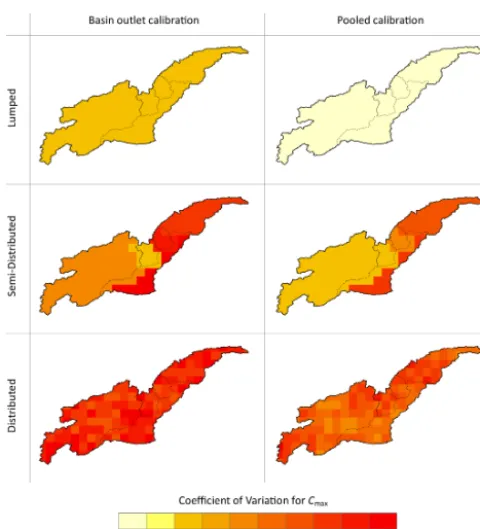
After reviewing all of the calibration experiments, it be-comes clear that the Semi-Pooled and Dist-Pooled calibra-tions provide more robust performance compared to the basin outlet calibrations due to their improved representation of in-ternal hydrologic processes across the basin. To further com-pare these calibration strategies against one another, we eval-uate the variability in optimal parameters resulting from the 50 trials of the GA algorithm. Figure 9 shows the coefficient of variation (CV) ofCmax(a parameter for the soil moisture account module) over the basin from all combinations of cal-ibration approaches (the outlet and pooled) and three param-eterization schemes. A clear pattern of increasing variabil-ity (higher uncertainty inCmax) emerges as parameter com-plexity increases for both the outlet and pooled calibration strategies. That is, the semi- and fully distributed parameter-izations lead to significantly variable parameter sets that pro-duce similar representations of the observed basin response. Figure 9 also suggests that the equifinality can be alleviated to an extent by pooling data across sites. The pooled calibra-tion approaches consistently show lower variability inCmax compared to the outlet calibration at the same level of param-eter complexity. These results are relatively consistent across the remaining 14 HYMOD_DS parameters. The implications of parameter stability on streamflow projections under cli-mate change is addressed in the next section.
5.4 Climate change projections of streamflow with uncertainty
Figure 9. Coefficient of variation (CV) of 50 optimal values of
Cmax(parameter for the soil moisture accounting module in the HYMOD_DS) from the basin outlet calibrations (left panel) and the pooled calibrations (right panel).
the CMIP5 GCM projections of monthly total precipitation and mean temperature are shown in Fig. S5. According to the CMIP5 ensemble, precipitation projections show no clear trend; the average precipitation change in monthly total pre-cipitation fluctuates between−10 and 10 mm. On the other hand, temperature clearly shows an upward trend for both radiative forcing scenarios. The average changes in annual temperature are +2.2 and +2.8◦C for RCPs 4.5 and 8.5, which, using the Hamon method, correspond to an increase in annual PET by approximately 100 and 150 mm, respec-tively.
We first examine average monthly streamflow estimates across four calibration strategies: the Semi-Pooled and Dist-Pooled (most promising calibration strategies), as well as the Lump-Outlet (as a baseline) and Dist-Outlet (the best outlet calibration strategy). Figure 10 shows the monthly stream-flow estimates for the historical period with the whisker bars indicating the uncertainty range across the 50 calibration tri-als. The monthly streamflow predictions are also provided for the 2050s under the RCP 4.5 and 8.5 scenarios. For the fu-ture scenarios, the whisker bars are derived by averaging over the 36 different climate projections for each of the 50 trials. For the historical time period, all calibration schemes match the observed monthly streamflow at Dakah well, but monthly streamflow is underestimated in most months at Kama and Asmar under the basin outlet calibrations, particularly by the
Lump-Outlet. The historical monthly streamflow estimates from the outlet calibration strategies also tends to be highly uncertain for the months of June, July, August, and Septem-ber, especially compared to the Semi-Pool and Dist-Pool.
Under future climate projections for the 2050s, the four calibration strategies show similar changes in monthly streamflow at Dakah, but the magnitudes of change are some-what different. All calibration strategies suggest reduction in streamflow for June, July, and August under both RCP 4.5 and 8.5 scenarios. Also, the peak monthly flow, which oc-curred in June or July in the historical period, is shifted to May at Dakah. However, the Lump-Outlet predicts less re-duction of flow in June and July and a greater rere-duction in August and September as compared to the other three cali-brations. Considering that all calibration schemes had simi-lar levels of good performance at this site for both calibration and validation periods, it is notable that they project future streamflow somewhat differently.
Future monthly streamflow predictions at Kama and As-mar vary widely between the four calibration schemes, mostly an artifact of their historic differences (Fig. 10). Streamflow projections under the outlet calibration strate-gies tend to show large uncertainties at these two sites, particularly the Lump-Outlet calibration. For three months, July–September, the outlet calibration and pooled calibra-tion strategies provide substantially different insights about future water availability at Kama and Asmar. The outlet cali-brations suggest less water with large uncertainties for those months as compared to the pooled calibrations. At Kama, the pooled calibrations suggest significant changes in the pattern of peak monthly flow timing under both RCP scenarios; in-stead of having a clear peak in July, streamflow from May to August show similar amounts of water.
To further understand the sources of uncertainty in future water availability, we evaluate the separate and joint influ-ence of uncertainties in parameter estimation and future cli-mate on seasonal streamflow projections across all calibra-tion schemes. Figure 11 represents the uncertainty of wet and dry seasonal streamflow at Dakah from three sources: (1) calibration uncertainty across the 50 trials, with future climate uncertainty averaged out for each trial; (2) future cli-mate uncertainty across the 36 projections, with calibration uncertainty averaged out across the 50 trials; and (3) the com-bined uncertainty across all 1800 (50×36) simulations. The results suggest somewhat surprisingly that uncertainty reduc-tion can be expected as parameter complexity increases and, less surprisingly, by applying pooled calibration approaches. Another clear point is that the uncertainty resulting from dif-ferent climate change scenarios substantially outweighs that from calibration uncertainty.
Figure 10. Historical and 2050s average monthly streamflow predictions at Dakah, Kama, and Asmar under four calibration strategies:
Lump-Outlet, Dist-Outlet, Semi-Pooled, and Dist-Pooled. The error bars represent the streamflow ranges resulting from 50 trails of the HYMOD_DS calibration. For each of the 50 trials, the 2050s streamflow predictions are averaged over 36 GCM climate projections.
Figure 11. Uncertainties in wet and dry season average streamflow predictions for 2050s are derived from the basin outlet and pooled
[image:14.612.128.469.428.631.2]flows from distributed models are noticeable (Reed et al., 2004) and spatial variability in model parameters signifi-cantly influence the runoff behavior (Brath and Montanari, 2000; Pokhrel and Gupta, 2011). The spatial variability of optimal parameters derived from the Semi-Pooled and Dist-Pooled is shown in Fig. S6, with larger variability across all parameters for the Dist-Pooled than for the Semi-Pooled. To understand the effects of spatial variability and calibration uncertainty of parameters on extreme event estimation, the 100-year daily flood event was calculated under the Semi-Pooled and Dist-Semi-Pooled for each of the 50 historic simula-tions and 1800 future simulasimula-tions across both RCP scenar-ios. Although the intermodel comparison is intended to be a useful addition that provides a distinction between the pa-rameterization schemes in the pooled calibration approach, results from this analysis should be viewed in the context of a theoretical calibration exercise, not for decision-making purposes, because no observed daily streamflow is avail-able against which to compare the estimated 100-year daily flood events. Projections of the 100-year daily flood, esti-mated using a log-Pearson type III distribution fit to annual peaks of 30 years, differ somewhat between the Semi-Pooled and Dist-Pooled (Fig. 12). At three validation sites, extreme floods are consistently larger under the Semi-Pooled than the Dist-Pooled, and the mean difference in the 100-year daily flood estimate between the two calibration approaches grows between the historic runs and the RCP 4.5 and 8.5 scenar-ios. This suggests that the flood-generation process is funda-mentally different between the two parameterizations, with the Semi-Pooled formalization magnifying the effect of cli-mate change on extremes. Furthermore, there is substantially more uncertainty in the 100-year daily flood estimate un-der the Semi-Pooled. Figure 12 shows the combined uncer-tainty across both climate projections and calibrations, but this uncertainty is broken down further in Fig. 13. Similar to Fig. 11, three sources of uncertainty are evaluated for the 100-year daily flood, including calibration uncertainty alone, climate projection uncertainty alone, and their combined ef-fect. For both the Semi-Pooled and Dist-Pooled, calibration uncertainty has a smaller influence than projection uncertain-ties and, for all sites, the Dist-Pooled has a smaller uncer-tainty range than the Semi-Pooled, even for calibration un-certainty alone. This was a truly surprising result, given the parametric freedom in the Dist-Pooled model and the fact that no daily data were ever used in the calibration of either model. It appears that a lack of model parsimony does not necessarily lead to greater uncertainty in model simulations under different climate conditions, somewhat counter to what would be expected of overfit models. One possible reason for this result would be if increased parametric freedom some-how offset the effects of structural deficiencies in the model. However, further research is needed to investigate this issue.
Figure 12. Comparison of GCM average 100-year daily flood
events derived from the semi-distributed and distributed pooled cal-ibrations. The uncertainty range is from 50 trials of the model cali-bration.
6 Discussion and conclusion
In this study we examined a variety of calibration experi-ments to better understand the benefits and costs associated with different calibration choices for a complex, distributed hydrologic model in a data-scarce region. The goal of these experiments was to provide insight regarding the use of mul-tisite data in calibration, the effects of parameter complexity, and the challenges of using limited data for distributed model calibration, all in the context of projecting future streamflow under climate change.
Figure 13. Uncertainties in 100-year daily flood estimates for 2050s
are assessed using the Semi-Pooled and Dist-Pooled calibrations. Uncertainties are evaluated by calculating the CV of the 2050s 100-year flood estimates under three uncertainty sources: calibration uncertainty across 50 calibration trials (Par), climate uncertainty across GCM projections (Clim), and combined uncertainty (Joint).
number of the HYMOD_DS parameters being calibrated in the semi-distributed approach remains realistic, but the fully distributed parameterization scheme likely causes poor iden-tifiability of the parameters. Thus, pursuing a parsimonious configuration (e.g., optimization for a small portion of the parameters) with an effort to increase the amount of informa-tion (e.g., multivariable/multisite) is critical in the calibrainforma-tion of watershed system models (Gupta et al., 1998; Efstratiadis et al., 2008). We also note the important role of experienced hydrologists in designing a parsimonious hydrologic calibra-tion (e.g., Boyle et al., 2000). In this study, the feasible ranges of the HYMOD_DS parameters were kept wide (as is often done in automatic hydrologic calibrations) without consider-ation of the physical properties of the basin; the judgment of local hydrologic experts could help reduce the feasible ranges used during the calibration and thus contribute to a reduction of calibration uncertainty.
Calibration only based on data at the basin outlet is all too common in hydrologic model applications and is sometimes considered comparable to multisite calibrations even for pre-dictions at interior gauges (Lerat et al., 2012). In contrast, others have reported improvements in interior flow predic-tions by using internal flow measurements (Anderson et al., 2001; Wang et al., 2012; Boscarello et al., 2013). This is in agreement with the findings from this study, demonstrating the superiority of the pooled calibration approach to the basin outlet calibration in terms of its ability to represent interior hydrologic response correctly. This study shows the danger in relying on an outlet calibration for interior flow prediction. It was shown that caution is needed when using an out-let calibration approach for streamflow predictions under fu-ture climate conditions. This study showed that the basin outlet calibration can lead to projections of mid-21st
cen-tury streamflow that deviate substantially from projections under multisite calibration strategies. From the test of impli-cations of the pooled calibration in the context of climate change, it was found that applying the pooled calibration with semi-distributed and distributed parameter formulations showed clear gains in reducing uncertainties in predictions of monthly and seasonal water availability as compared to the basin outlet calibrations. Surprisingly, increased parameter complexity in the calibration strategies did not increase the uncertainty in streamflow projections, even though parame-ter equifinality did emerge. The results suggest that increased (excessive) parameter complexity does not always lead to in-creased uncertainty if structural uncertainties in the model are present.
The semi-distributed pooled and distributed pooled cali-brations are very similar for monthly streamflow projections, yet differ in their projections of extreme flows in part due to their differences in the spatial variability of optimal parame-ters, with the distributed pooled calibration showing less un-certainty for 100-year daily flood events. We evaluated the separate and joint influence of uncertainties in parameter esti-mation and future climate on projections of seasonal stream-flow and 100-year daily flood across calibration schemes and found that the uncertainty resulting from variations in pro-jected climate between the CMIP5 GCMs substantially out-weighs the calibration uncertainty. These results agree with other studies showing the dominance of GCM uncertainty in future hydrologic projections (Chen et al., 2011; Exbrayat et al., 2014). While the GCM-based simulations still have widespread use in assessing the impacts of climate change on water resources availability, the bounds of uncertainty re-sulting from an ensemble of GCMs cannot be well-defined because of the low credibility with which GCMs are able to produce time series of future climate (Koutsoyiannis et al., 2008). This issue hinders a straightforward appraisal of future water availability under climate change and has mo-tivated other efforts; e.g., performance-based selection of GCMs (Perez et al., 2014).
In addition to the uncertainties surrounding model param-eters and future climate explored in this study, there is also significant uncertainty in streamflow projections stemming from structural differences between applied hydrologic mod-els, which can be especially pertinent where robust calibra-tion is hampered by the scarcity of data (Exbrayat et al., 2014). Furthermore, the residual error variance of hydrologic model simulations would increase the effects of hydrologic model uncertainty as compared to that of the climate projec-tions (Steinschneider et al., 2014). These issues need to be addressed in future work for exploring a comprehensive un-certainty assessment of climate change risk for poorly moni-tored hydrologic systems.
Although the speed and capacity of computers have in-creased multifold in the past several decades, the time con-sumed by running hydrological models (especially complex, physically based, distributed hydrological models) is still a concern for hydrology practitioners. A single trial of param-eter optimization of HYMOD_DS associated with 100 000 runs can take 28 days on a single processor (Fig. S7). Ac-cordingly, the use of high-performance computing power was essential in this study to better understand the impli-cations of different calibration choices and their associated uncertainty for streamflow projections. Enhanced data with high spatial and temporal resolution are increasingly avail-able from remote sensing and satellite products. In the future, remote sensing and satellite information can be integrated into calibration approaches to develop more robust estimates of spatially distributed parameter values, enabling internal consistency of distributed hydrological modeling. Significant progress has been made toward this end (Tang et al., 2009; Khan et al., 2011; Thirel et al., 2013). Future work will con-sider using high-performance computing power (e.g., Laloy and Vrugt, 2012; Zhang et al., 2013) to understand how such information can enhance the hydrologic simulation at ungaged sites and reduce the calibration uncertainty of dis-tributed hydrologic models in data-scarce regions.
The Supplement related to this article is available online at doi:10.5194/hess-19-857-2015-supplement.
Acknowledgements. The authors are grateful to Efrat Morin,
An-dreas Efstratiadis, and one anonymous reviewer for their construc-tive suggestions for improving this manuscript.
This research is funded by a World Bank grant: Hydro-Economic Modeling for Brahmaputra and Kabul River. The views expressed in this paper are those of the authors and do not necessarily reflect the views of the World Bank.
We acknowledge the use of the supercomputing facilities managed by the Research Computing department at the University of Massachusetts.
Edited by: E. Morin
References
Ahmad, S.: Towards Kabul Water Treaty: Managing Shared Water Resources – Policy Issues and Options, Karachi, Pakistan, 2010. Ajami, N. K., Gupta, H., Wagener, T., and Sorooshian, S.: Calibra-tion of a semi-distributed hydrologic model for streamflow esti-mation along a river system, J. Hydrol., 298, 112–135, 2004. Anderson, J., Refsgaard, J. C., and Jensen, K. H.: Distributed
hydro-logical modeling of the Senegal river basin – model construction and validation, J. Hydrol., 247, 200–214, 2001.
Bandaragoda, C., Tarboton, D. G., and Woods, R.: Application of TOPNET in the distributed model intercomparison project, J. Hydrol., 298, 178–201, 2004.
Beven, J. K.: Rainfall-Runoff Modelling: The Primer, 2nd Edition, Wiley-Blackwell, Chichester, 2012.
Beven, K. and Freer, J.: Equifinality, data assimilation, and uncer-tainty estimation in mechanistic modelling of complex environ-mental systems using the GLUE methodology, J. Hydrol., 249, 11–29, 2001.
Beven, K.: How far can we go in distributed hydrological mod-elling?, Hydrol. Earth Syst. Sci., 5, 1–12, doi:10.5194/hess-5-1-2001, 2001.
Biondi, D., Freni, G., Iacobellis, V., Mascaro, G., and Montanari, A.: Validation of hydrological models: conceptual basis, method-ological approaches and a proposal for a code of practice, Phys. Chem. Earth, 42–44, 70–76, 2012
Boscarello, L., Ravazzani, G., and Mancini, M.: Catchment multi-site discharge measurements for hydrological model calibration, Procedia Environmental Sciences, 19, 158–167, 2013.
Boyle, D. P., Gupta, H. V., and Sorooshian, S.: Toward improved calibration of hydrologic models: Combining the stregths of manual and automatic methods, Water Resour. Res., 36, 3663– 3674, 2000.
Boyle, D. P.: Multicriteria calibration of hydrologic models, Ph.D. thesis, Department of Hydrology and Water Resources Engineer-ing, The University of Arizona, USA, 2001.
Brath, A. and Montanari, A.: The effects of the spatial variability of soil infiltration capacity in distributed flood modelling, Hydrol. Process., 14, 2779–2794, 2000.
Brath, A., Montanari, A., and Toth, E.:. Analysis of the effects of different scenarios of historical data availability on the cali-bration of a spatially-distributed hydrological model, J. Hydrol., 291, 232–253, 2004.
Breuer, L., Huisman J. A., Willems, P., Bormann, H., Bronstert, A., Croke, B. F. W., Frede, H. G., Gräff, T., Hubrechts, L., Jakeman, A. J., Kite, G., Lanini, J., Leavesley, G., Lettenmaier, D. P., Lind-ström, G., Seibert, J., Sivapalan, M., and Viney, N. R.: Assessing the impact of land use change on hydrology by ensemble model-ing (LUChEM). I: Model intercomparison with current land use, Adv. Water Resour., 32, 129–146, 2009
Cao, W., Bowden, W. B., Davie, T., and Fenemor, A.: Multi-variable and multi-site calibration and validation of SWAT in a large mountainous catchment with high spatial variability, Hydrol. Process, 20, 1057–1073, 2006.
Chen, J., Brissette, F. P., Poulin, A., and Leconte, R.: Overall un-certainty study of the hydrological impacts of climate change for a Canadian watershed, Water Resour. Res., 47, W12509, doi:10.1029/2011WR010602, 2011.
Cole, S. J. and Moore, R. J.: Hydrological modelling using raingauge- and radar-based estimators of areal rainfall, J. Hy-drol., 358, 159–181, 2008.
DAWN: Pakistan, Afghanistan mull over power project on Kunar River, available at: http://www.dawn.com/news/1038435 (last access: 2 January 2015), 2013.
Eckhardt, K., Fohrer, N., and Frede, H. G.: Automatic model cali-bration, Hydrol. Process., 19, 651–658, 2005.
Efstratiadis, A. and Koutsoyiannis, D.: One decade of multi-objective calibration approaches in hydrological modelling: a re-view, Hydrolog. Sci. J., 55, 58–78, 2010.
Earth Syst. Sci., 12, 989–1006, doi:10.5194/hess-12-989-2008, 2008.
Exbrayat, J. F., Buytaert, W., Timbe, E., Windhorst, D., and Breuer, L.: Addressing sources of uncertainty in runoff projections for a data scarce catchment in the Ecuadorian Andes, Climatic Change, 125, 221–235, 2014.
Flugel, W. A.: Delineating Hydrological Response Units (HRU’s) by GIS analysis for regional hydrological modelling using PRMS/MMS in the drainage basin of the River Brol, Germany, Hydrol. Process., 9, 423–436, 1995.
Forsythe, W. C., Rykiel Jr., E. J., Stahl, R. S., Wu, H., Schoolfield, R. M.: A model comparison for daylength as a function of lati-tude and day of year, Ecol. Model., 80, 87–95, 1995.
Frances, F., Velez, J. I., and Velez, J. J.: Split-parameter structure for the automatic calibration of distributed hydrological models, J. Hydrol., 332, 226–240, 2007.
Gharari, S., Hrachowitz, M., Fenicia, F., and Savenije, H. H. G.: An approach to identify time consistent model parameters: sub-period calibration, Hydrol. Earth Syst. Sci., 17, 149–161, doi:10.5194/hess-17-149-2013, 2013.
Grinsted, A.: An estimate of global glacier volume, The Cryosphere, 7, 141–151, doi:10.5194/tc-7-141-2013, 2013. Gupta, H. V., Kling, H., Yilmaz, K. K., and Martinez, G. F.:
Decom-position of the mean squared error and NSE performance criteria: Implications for improving hydrological modelling, J. Hydrol., 377, 80–91, 2009.
Gupta, H. V., Sorooshian, S., and Yapo, P. O.: Towards improved calibration of hydrologic models: Multiple and noncommensu-rable measures of information, Water Resour. Res., 34, 751–763, 1998.
Hamon, W. R.: Estimating potential evapotranspiration, J. Hydr. Eng. Div.-ASCE, 87, 107–120, 1961.
Hewitt, K., Wake, C. P., Young, G. J., and David, C.: Hydrologicl investigations at Biafo glacier, Karakoram Himalaya, Pakistan: An important source of water for the Indue River, Ann. Glaciol., 13, 103–108, 1989.
Immerzeel, W. W., van Beek, L. P. H., Konz, M., Shrestha, A. B., and Bierkens, M. F. P.: Hydrological response to climate change in a glacierized catchment in the Himalayas, Climatic Change, 110, 721–736, 2012.
IUCN: Towards Kabul Water Treaty: Managing Shared Water Re-sources – Policy Issues and Options, IUCN Pakistan, Karachi, 11 pp., 2010.
Jarvis, A., Reuter, H. I., Nelson, A., and Guevara, E.: Hole-filled seamless SRTM data V4, International Centre for Tropical Agri-culture (CIAT), available at: http://srtm.csi.cgiar.org (last access: 2 January 2015), 2008.
Khakbaz, B., Imam, B., Hsu, K., and Sorooshian, S.: From lumped to distributed via semi-distributed: Calibration strategies for semi-distributed hydrologic models, J. Hydrol., 418–419, 61–77, 2012.
Khan, S. I., Yang, H., Wang, J., Yilmaz, K. K., Gourley, J. J., Adler, R. F., Brakenridge, G. R., Policell, F., Habib, S., and Irwin, D.: Satellite remote sensing and hydrologic modeling for flood inun-dation mapping in Lake Victoria Basin: Implications for hydro-logic prediction in ungauged basins, IEEE T. Geosci. Remote, 49, 85–95, 2011.
Kinouchi, T., Liu, T., Mendoza, J., and Asaoka, Y.: Modeling glacier melt and runoff in a high-altitude headwater catchment in the
Cordillera Real, Andes, Hydrol. Earth Syst. Sci. Discuss., 10, 13093–13144, doi:10.5194/hessd-10-13093-2013, 2013. Kollat, J. B., Reed, P. M., and Wagener, T.: When are multiobjective
calibration trade-offs in hydrologic models meaningful?, Water Resour. Res., 48, W03520, doi:10.1029/2011WR011534, 2012. Konz, M. and Seibert, J.: On the value of glacier mass balances for
hydrological model calibration, J. Hydrol., 385, 238–246, 2010. Koren, V., Reed, S., Smith, M., Zhang, Z., and Seo, D. J.: Hydrol-ogy laboratory research modeling system (HL-RMS) of the US national weather service, J. Hydrol., 291, 297–318, 2004. Koutsoyiannis, D., Efstratiadis, A., Mamassis, N., and Christofides,
A.: On the credibility of climate predictions, Hydrolog. Sci. J., 53, 671–684, 2008.
Kumar, R., Samaniego, L., and Attinger, S.: Implications of dis-tributed hydrologic model parameterization on water fluxes at multiple scales and locations, Water Resour. Res., 49, 360–379, 2013.
Kuzmin, V., Seo D., and Koren V.: Fast and efficient optimization of hydrologic model parameters using a priori estimates and step-wise line search, J. Hydrol., 353, 109–128, 2008.
Laloy, E. and Vrugt, J. A.: High-dimensional posterior explo-ration of hydrologic models using multiple-try DREAM(ZS) and high-performance computing, Water Resour. Res., 48, W01526, doi:10.1029/2011WR010608, 2012.
Latham, J., Cumani, R., Rosati, I., and Bloise, M.: Global Land Cover SHARE (GLC-SHARE) database Beta-Release Version 1.0, available at: http://www.glcn.org/databases/lc_glcshare_en. jsp (last access: 2 January 2015), 2014.
Leavesley, G. H., Hay, L. E., Viger, R. J., and Markstrom, S. L.: Use of Priori Paramter-Estimation Methods to Constrain Calibration of Distributed-Parameter Models, Water. Sci. Appl., 6, 255–266, 2003.
Legates, D. R. and Willmott, C. J.: Mean seasonal and spatial vari-ability in gauge-corrected, global precipitation, Int. J. Climatol., 10, 111–127, 1990.
Lerat, J., Andreassian V., Perrin, C., Vaze, J., Perraud J. M., Rib-stein, P., and Loumagne C.: Do internal flow measurements im-prove the calibration of rainfall-runoff models?, Water Resour. Res., 48, W02511, doi:10.1029/2010WR010179, 2012. Li, X., Weller, D. E., and Jordan, T. E.: Watershed model calibration
using multi-objective optimization and multi-site averaging, J. Hydrol., 380, 277–288, 2010.
Lohmann, D., Raschke, R., Nijssen, B., and Lettenmaier, D. P.: Re-gional scale hydrology: I. Formulation of the VIC-2L model cou-pled to a routing model, Hydrolog. Sci. J., 43, 131–141, 1998. Madsen, H.: Parameter estimation in distributed hydrologicl
catch-ment modelling using automatic calibration with multiple objec-tives, Adv. Water Resour., 26, 205–216, 2003.
Moore, R. D.: Application of a conceptual streamflow model in a glacierized drainage basin, J. Hydrol., 150, 151–168, 1993. Moore, R. J.: The probability-distribted principle and runoff
pro-duction at point and basin scales, Hydrolog. Sci. J., 30, 273–297, 1985.
Nash, J. E. and Sutcliff, J. V.: River flow forecasting through con-ceptual models: Part 1. A discussion of priciples, J. Hydrol., 10, 282–290, 1970.
Olson, S. A. and Williams-Sether, T.: Streamflow characteristics at streamgages in Northern Afghanistan and selected locations, U.S. Geological Survey, Reston, Virginia, 2010.
Palazzi, E., von Hardenberg, J., and Provenzale, A.: Precipitation in the Hindu-Kush Karakoram Himalaya: Observations and future scenarios, J. Geophys. Res., 118, 85–100, 2013.
Perez, J., Menendez, M., Mendez, F. J., and Losada, I. J.: Evaluat-ing the performance of CMIP3 and CMIP5 global climate mod-els over the north-east Atlantic region, Clim. Dynam., 43, 2663– 2680, 2014.
Pfeffer, T. W., Arendt, A. A., Bliss, A., Bolch, T., Cogley J. G., Gardner, A. S., Hagen, J. O., Hock R., Kaser, G., Kienholz, C., Miles E. S., Moholdt, G., Molg, N., Paul, F., Radic, V., Rastner, P., Raup, B. H., Rich, J., Sharp, M. J., and The Randolph Consor-tium: The Randolph Glacier Inventory, J. Glaciol., 60, 537–552, 2014.
Pokhrel, P. and Gupta, H. V.: On the use of spatial regularization strategies to improve calibration of distributed watershed models, Water. Resour. Res., 46, W01505, doi:10.1029/2009WR008066, 2010.
Pokhrel, P. and Gupta, H. V.: On the ability to infer spatial catch-ment variability using streamflow hydrographs, Water Resour. Res., 47, W08534, doi:10.1029/2010WR009873, 2011. Radic, V., Bliss, A., Beedlow, A. C., Hock, R., Miles, E., and
Cog-ley, J. G.: Regional and global projections of twenty-first cen-tury glacier mass changes in response to climate scenarios from global climate models, Clim. Dynam., 42, 37–58, 2014. Reed, S., Koren, V., Smith, M., Zhang, Z., Moreda, F., Seo, D. J.,
and DMIP Participants: Overall distributed model intercompari-son project results, J. Hydrol., 298, 27–60, 2004.
Remesan, R., Bellerby, T., and Frostick, L.: Hydrological modelling using data from monthly GCMs in a regional catchment, Hydrol. Process., 28, 3241–3263, 2013.
Safari, A., De Smedt, F., and Moreda, F.: WetSpa model application in the Distributed Model Intercomparison Project (DMIP2), J. Hydrol., 418–419, 77–89, 2012.
Shakir, A. S., Rehman, H., and Ehsan, S.: Climate change impact on river flows in Chitral watershed, Pakistan Journal of Engineering and Applied Sciences, 7, 12–23, 2010.
Smith, M. B., Koren, V., Reed, S., Zhang, Z., Zhang, Y., Moreda, F., Cui, Z., Mizukami, N., Anderson, E. A., and Cosgrove, B. A.: The distributed model intercomparison project – Phase 2: Moti-vation and design of the Oklahoma experiments, J. Hydrol., 418– 419, 3–16, 2012.
Smith, M. B., Seo, D. J., Koren, V. I., Reed, S. M., Zhang, Z., Duan, Q., Moreda, F., and Cong, S.: The distributed model intercom-parison project (DMIP): motivation and experiment design, J. Hydrol., 298, 4–26, 2004.
Smith, M., Koren, V., Zhang, Z., Moreda, F., Cui, Z., Cosgrove, B., Mizukami, N., Kitzmiller, D., Ding, F., Reed, S., Anderson, E., Schaake, J., Zhang, Y., Andreassian, V., Perrin, C., Coron, L., Valery, A., Khakbaz, B., Sorooshian, S., Behrangi, A., Imam, B., Hsu, K. L., Todini, E., Coccia, G., Mazzetti, C., Andres, E. O., Frances, F., Orozco, I., Hartman, R., Henkel, A., Fickenscher, P., and Staggs, S.: The distributed model intercomparison project – Phase 2: Experiment design and summary results of the western basin experiments, J. Hydrol., 507, 300–329, 2013.
Stahl, K., Moore, R. D., Shea, J. M., Hutchinson, D., and Cannon, A. J.: Coupled modelling of glacier and streamflow response
to future climate scenarios, Water Resour. Res., 44, W02422, doi:10.1029/2007WR005956, 2008.
Steinschneider, S., Polebitski, A., Brown, C., and Letcher, B. H.: Toward a statistical framework to quantify the uncertainties of hydrologic response under climate change, Water Resour. Res., 48, W11525, doi:10.1029/2011WR011318, 2012.
Steinschneider, S., Wi, S., and Brown, C.: The integrated effects of climate and hydrologic uncertainty on future flood risk as-sessments, Hydrol. Process., doi:10.1002/hyp.10409, accepted, 2014.
Talyor, K. E., Stouffer, R. J., and Meehl, G. A.: An Overview of CMIP5 and the Experiment Design, B. Am. M. Soc., 93, 485– 498, 2012.
Tang, Q., Gao, H., Lu, H., and Lettenmaier, D. P.: Remote sensing: hydrology, Prog. Phys. Geog., 33, 490–509, 2009.
Thirel, G., Salamon, P., Burek, P., and Kalas, M.: Assimilation of MODIS snow cover area data in a distributed hydrological model using the particle filter, Remote Sensing, 5, 5825–5850, 2013 USDA-NRCS: FAO-UNESCO Soil Map of the World,
avail-able at: http://www.nrcs.usda.gov/wps/portal/nrcs/detail/soils/ use/?cid=nrcs142p2_054013 (last access: 2 January 2015), 2005. Vrugt, J. A., ter Braak, C. J. F., Gupta, H. V., and Robinson, B. A.: Equifinality of formal (DREAM) and informal (GLUE) Bayesian approaches in hydrologic modeling?, Stoch. Env. Res. Risk A., 23, 1011–1026, 2008.
Wagener, T., Boyle, D. P., Lees, M. J., Wheater, H. S., Gupta, H. V., and Sorooshian, S.: A framework for development and applica-tion of hydrological models, Hydrol. Earth Syst. Sci., 5, 13–26, doi:10.5194/hess-5-13-2001, 2001.
Wagener, T., Wheater, H. S., and Gupta, H. V.: Rainfall-Runoff Modelling in Gauged and Ungauged Catchments, Imperical Col-lege Press, London, 2004.
Wang, Q. J.: The Genetic Algorithm and Its Application to Calibrat-ing Conceptual Rainfall-Runoff Models, Water Resour. Res., 27, 2467–2471, 1991.
Wang, S., Zhang, Z., Sun, G., Strauss, P., Guo, J., Tang, Y., and Yao, A.: Multi-site calibration, validation, and sensitivity analysis of the MIKE SHE Model for a large watershed in northern China, Hydrol. Earth Syst. Sci., 16, 4621–4632, doi:10.5194/hess-16-4621-2012, 2012.
Wilby, R. L.: Uncertainty in water resource model parameters used for climate change impact assessment, Hydrol. Process., 19, 3201–3219, 2005.
Wood, A. W., Leung, L. R., Sridhar, V., and Lettenmaier, D. P.: Hy-drologic Implications of Dynamical and Statistical Approaches to Downscaling Climate Model Outputs, Climatic Change, 62, 189–216, 2004.
World Bank: Afghanistan – Scoping strategic options for develop-ment of the Kabul River Basin: a multisectoral decision support system approach, World Bank, Washington, D.C., 2010. Yatagai, A., Kamiguchi, K., Arakawa, O., Hamada, A., Yasutomi,
N., and Kitoh, A.: APHRODITE: Constructing a Long-Term Daily Gridded Precipitation Dataset for Asia Based on a Dense Network of Rain Gauges, B. Am. Meteorol. Soc., 93, 1401–1415, 2012.
Zhang, X., Beeson, P., Link, R., Manowitz, D., Izaurralde, R. C., Sadeghi, A., Thomson, A. M., Sahajpal, R., Srinivasan, R., and Arnold, J. G.: Efficient multi-objective calibration of a computa-tionally intensive hydrologic model with parallel computing soft-ware in Python, Environ. Modell. Softw., 46, 208–218, 2013.