ScholarWorks @ Georgia State University
ScholarWorks @ Georgia State University
Computer Science Dissertations Department of Computer Science
Spring 3-9-2012
Shadow Price Guided Genetic Algorithms
Shadow Price Guided Genetic Algorithms
Gang Shen
Georgia State University
Follow this and additional works at: https://scholarworks.gsu.edu/cs_diss
Recommended Citation Recommended Citation
Shen, Gang, "Shadow Price Guided Genetic Algorithms." Dissertation, Georgia State University, 2012. https://scholarworks.gsu.edu/cs_diss/64
This Dissertation is brought to you for free and open access by the Department of Computer Science at
by
GANG SHEN
Under the Direction of Yan-Qing Zhang
ABSTRACT
The Genetic Algorithm (GA) is a popular global search algorithm. Although it has been used
successfully in many fields, there are still performance challenges that prevent GA’s further
success. The performance challenges include: difficult to reach optimal solutions for complex
problems and take a very long time to solve difficult problems. This dissertation is to research
new ways to improve GA’s performance on solution quality and convergence speed. The main
focus is to present the concept of shadow price and propose a two-measurement GA. The new
algorithm uses the fitness value to measure solutions and shadow price to evaluate components.
New shadow price Guided operators are used to achieve good measurable evolutions. Simulation
results have shown that the new shadow price Guided genetic algorithm (SGA) is effective in
terms of performance and efficient in terms of speed.
by
GANG SHEN
A Dissertation Submitted in Partial Fulfillment of the Requirements for the Degree of
Doctor of Philosophy
in the College of Arts and Sciences
Georgia State University
Copyright by Gang Shen
by
GANG SHEN
Committee Chair: Yan-Qing Zhang
Committee: Raj Sunderraman
YingShu Li
Yichuan Zhao
Electronic Version Approved:
Office of Graduate Studies
College of Arts and Sciences
Georgia State University
ACKNOWLEDGMENTS
I thank my advisor, Dr. Yan-Qing Zhang, for his guidance and help for my Ph.D. study. I truly
appreciate the time and patience he spend helping me completing the program in research,
publishing, and dissertation work. I also thank Dr. Rajshekhar Sunderraman for advising
throughout my study and being a member of dissertation committee. I am grateful for Dr.
TABLE OF CONTENTS
ACKNOWLEDGMENTS iv
TABLE OF CONTENTS v
LIST OF TABLES viii
LIST OF FIGURES x
LIST OF ABBREVIATIONS xi
CHAPTER 1 INTRODUCTION 1
CHAPTER 2 IMPORTANCE OF THE RESEARCH 4
CHAPTER 3 GENETIC ALGORITHM 6
3.1 Principles of Genetic Algorithm 6
3.2 Opportunities 11
CHAPTER 4 RELATED WORK 13
4.1 Transforming Problem 13
4.2 Improving GA Operators 14
4.3 Adding Local Search 15
4.4 Hybriding with Other Algorithms 17
4.5 Using Parallel Processing 19
4.6 Miscellaneous Approaches 25
CHAPTER 5 DUALITY AND SHADOW PRICE in LINEAR PROGRAMMING 27
5.1 Definition 27
5.2 Shadow Prices in Linear Programming 29
6.1 The Concept 32
6.2 A Simple Example 34
6.3 Define Shadow Price 38
6.4 The Complete Algorithm 40
CHAPTER 7 OPTIMIZING THE TRAVELING SALESMAN PROBLEM WITH SGA 42
7.1 Introduction 42
7.2 Problem Definition 42
7.3 Shadow Price Definition 43
7.4 Shadow Price Guided Mutation Operator 45
7.5 Shadow Price Guided Crossover Operator 46
7.6 Solution Validation 46
7.7 Other Techniques 48
7.8 Experiments 49
7.9 Summary 50
CHAPTER 8 OPTIMIZING THE CUTTING STOCK PROBLEM WITH SGA 51
8.1 Introduction 51
8.2 Problem Definition 52
8.3 Basic Terminologies 54
8.4 Shadow Price Definition 55
8.5 Shadow Price Guided Mutation Operator 56
8.6 Shadow Price Guided Crossover Operator 58
8.7 Experiments 59
8.8 Results Analysis 69
8.9 Production Consideration 71
CHAPTER 9 OPTIMIZING THE GREEN COMPUTING PROBLEMS WITH SGA 73
9.1 Introduction 73
9.2 Problem Definition 76
9.3 Shadow Price Guided GA Operator for P1 80
9.4 Shadow Price Guided GA Operator for P2 82
9.5 Experiments for P1 87
9.6 Experiments for P2 91
9.7 Summary 95
CHAPTER 10 OPTIMIZING THE STOCK REDUCTION PROBLEM WITH SGA 95
10.1 Introduction 95
10.2 Problem Definition 97
10.3 LP/GA Hybrid Algorithm 98
10.4 Experiments 106
10.5 Summary 107
CHAPTER 11 CONCLUSION AND FUTURE WORK 109
11.1 Conclusion 109
11.2 Future Work 110
LIST OF TABLES
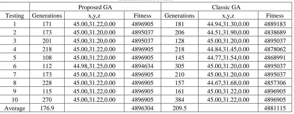
Table 6.1 Simulation results 37
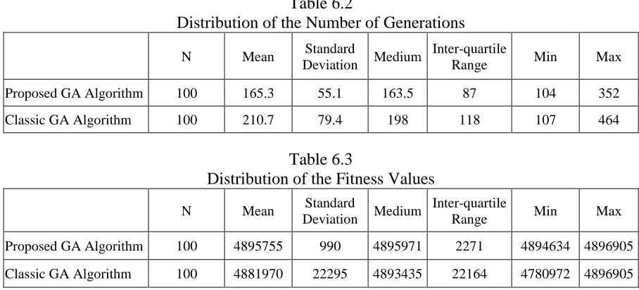
Table 6.2 Distribution of the Number of Generations 38
Table 6.3 Distribution of the Fitness Values 39
Table 7.1 Distance Matrix for gr17.tsp 44
Table 7.2 Comparison with the Ray, Bandyopadhyay, and Pal (2004) 49
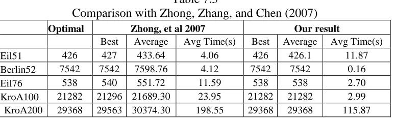
Table 7.3 Comparison with the Zhong, Zhang, and Chen 50
Table 7.4 Comparison with the Wong, Low, and Chong (2008) 50
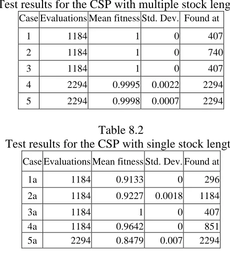
Table 8.1 Test results for the CSP with multiple stock lengths 53
Table 8.2 Test results for the CSP with single stock length 53
Table 8.3 Sample problem, the stock length is 14 54
Table 8.4 Test case summary 63
Table 8.5 Mean Fitness Value Comparison 63
Table 8.6 Total Waste Comparison 65
Table 8.7 Number of Stocks with Waste Comparison 66
Table 8.8 Speed Comparison 68
Table 8.9 Mean fitness value and number of stocks used 72
Table 8.10 Total waste, number of stocks with waste, and distinct pattern count 72
Table 9.1 A Sample Task Schedule 77
Table 9.2 Published Processor Specification 88
Table 9.3 Energy Consumption Comparison 89
Table 9.5 SPGA Time Improvement over GA for 10 Processors 93
Table 9.6 SPGA Time Improvement over GA for 20 Processors 93
Table 9.7 SPGA Time Improvement over GA for 30 Processors 93
Table 9.8 SPGA Time Improvement over GA for 40 Processors 93
Table 9.9 SPGA Time Improvement over GA for 50 Processors 94
Table 9.10 SPGA Search Speed Improvement in Time(s) 94
Table 9.11 SPGA Search Speed Improvement in Generations 94
Table 10.1 Sample CSP 101
Table 10.2 GA Result of Sample CSP 101
Table 10.3 Result from Using the Gilmore and Gomory LP Algorithm 102
Table 10.4 Convert LP Solutions to Integer Using Stock 1376 103
Table 10.5 Convert LP Solutions to Integer Using Stock 1392 103
Table 10.6 Comparison Study on Item Variations 106
Table 10.7 Comparison Study on Stock Count Variations 106
LIST OF FIGURES
Figure 3.1 Genetic Algorithm 10
Figure 5.1 Gilmore and Gomory LP Algorithm 31
Figure 6.1 New GA Framework with Shadow Price Guided Operators 40
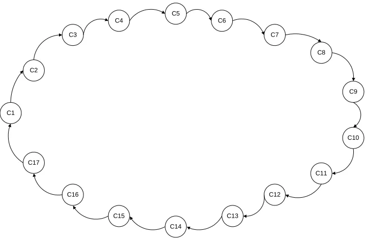
Figure 7.1 A Sample Tour 47
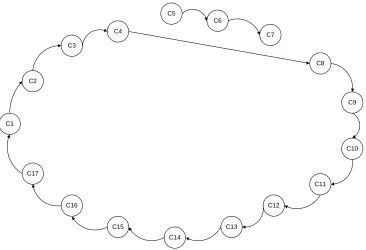
Figure 7.2 Result from Mutation 48
Figure 8.1 Algorithm B’s mutation operator 60
Figure 8.2 Algorithm C’s mutation operator 61
Figure 8.3 Algorithm D’s mutation operator 62
Figure 8.4 Average Mean Fitness Value Comparison 64
Figure 8.5 Maximum Mean Fitness Value Comparison 64
Figure 8.6 Average Total Waste Comparison 65
Figure 8.7 Minimum Total Waste Comparison 66
Figure 8.8 Average Number of Stocks with Waste Comparison 67
Figure 8.9 Minimum Number of Stocks with Waste Comparison 67
Figure 8.10 Best Solution Found Generation Comparison 68
LIST OF ABBREVIATIONS
Adaptive Hill-Climbing Crossover Local Search AHCXLS
Ant Colony Optimization ACO
Bee Colony Optimization BCO
Cutting Stock Problem CSP
Discrete Particle Swarm Optimization DPSO
Evolutionary Algorithm EA
Field Programmable Gate Array FPGA
Genetic Algorithm GA
Group Crossover BPCX
Infeasibility Driven Evolutionary Algorithm IDEA
Integer Linear Programming ILP
KiloWatt-Hours kWh
Linear Programming LP
Million Instructions Per Second MIPS
Minimizing Stock Mix Problem MSMP
Mixed Integer Linear Programming MILP
Mixed Integer Programming MIP
Neural Network NN
Parallel Genetic Algorithm PGA
Particle Swarm Optimization PSO
Shadow Price Guided GA SGA
Stock Reduction Problem SRP
System on a Programmable Chip SOPC
Traveling Salesman Problem TSP
CHAPTER 1 INTRODUCTION
Optimization is to search for the best solution from a domain of feasible solutions. In the
simplest form, it is to find the minimal or maximal value of a function while satisfying a set of
constraints. It is a process of searching for the best solutions using certain algorithms and
techniques. One most cited example of optimization is to find the best way to achieve maximum
profits utilizing limited resources.
Integer optimization is a special branch of general optimization that requires integer
solutions for the problem. This constraint only limits the final result in integer and does not pose
integer requirement to intermediate solutions. Thus, the intermediate solution can be in integer or
real. This constraint is often modeled from real life problems. For example, job scheduling is an
integer optimization problem; product can only be produced in integer units.
Other complicated constraints in optimizations include, complex objective functions,
multiple objectives optimization, etc. Objective functions can be linear, polynomial, table
lookup, etc. There can be multiple objective functions to be optimized in the same time.
Linear programming (LP) is the classic optimization algorithm. It is very efficient and
widely used in production especially for large complex linear optimization problems. But it is
limited to linear objective functions and constrains. The general LP results are in fractions.
Integer linear programming (ILP) and Mixed Integer Linear Programming (MIP) are special
cases of LP that provide integer solutions. Although they can solve many practical problems, ILP
and MIP are less efficient than LP and difficult to solve. Both ILP and MIP are extensions of
classic LP. They typically follow classic LP technique and add additional steps, algorithms (such
commonly used in the algorithms’ intermediate solutions and these fractional intermediate
solutions are not valid solutions.
Genetic Algorithm (GA) (John Holland, 1975, 1992) is a bio-inspired global search
algorithm that mimics nature’s evolution process. It is a multi-point, reward-based search
algorithm. In the search process, there are multiple valid solutions evolving forward together.
The reward-based search refers to the fact that only elite solutions participating next generation’s
evolution. It’s an integer intrinsic search process that fits integer optimization problem very well.
Unlike invalid fractional intermediate solutions in the LP search process, every solution in GA’s
search process are valid integer solutions although they may not be the optimal solutions. The
reward-based approach also suits for multi-objective optimizations since the elitism only requires
comparing the objective function regardless the function is linear or non-linear.
GA has been used successfully in many fields. Recent survey suggests that at least
thirty-six human-competitive results were produced by genetic programming (Koza et al. 2005). It is a
very straightforward algorithm and can be implemented rather quickly.
The challenges for GA’s performances are solution quality and search time. These two
concerns impede the practical applications of the algorithm. GA is a population based search
algorithm and there are many solutions in each generation. Solutions in the generation need to be
involved in one or more evolution operations in each generation to move forward. Based on the
size of the population, huge amount of calculation may be needed for each generation.
Compound with necessary randomness in the search process, GA can take very long time to find
optimal solutions.
Furthermore, GA may not always provide the optimal solutions. GA generally depends
is to limit the maximum number of generations, maximum allowed searching time, or solution
reaches acceptable quality. GA cannot prove the final solution is optimal or not. So, there is
certain randomness in the quality of the final solutions.
My research focuses on improving GA’s performance in both solution quality and search
speed. GA only measures the solution fitness value. The evolution operators are mostly
randomly applied since there is no measurement on the components. I propose using the
“Shadow Price” concept to measure the components of the solution in the GA search process. I
can improve GA operators using the shadow price. Thus, I establish a two-measurement GA.
The fitness value is used to measure solution and the shadow price is used to measure component
CHAPTER 2 IMPORTANCE OF THE RESEARCH
There are tremendous social and economic values in finding optimal solutions. The value
of best utilizing limited resources to maximize social benefit can be seen in daily life or in the
event of disaster. For example, it is very important to most efficiently use limited transportation
equipment and crew to move stranded passengers in the event of large-scale flight interruption
such as that caused by volcano eruptions, terrorist attacks, etc.
Significant economic value of optimization is everywhere. For example, trimming rolls
for paper machine is a typical optimization problem and referred as the cutting stock problem
(CSP). The goal is to improve trim efficiency. A 300 inch wide paper machine can produce half
million tons of medium weight paper a year. If the price is 600 dollars per ton, the total value of
the paper is 300 million dollars. A one percent trim efficiency improvement is equivalent to 3
million dollars a year for this machine. In a paper box plant, trimming corrugator is another CSP
and the trim efficiency improvement worth even more since it trims multiple layers of paper. For
a medium sized paper product company that operates multiple paper machines and paper box
plants, a minor trim efficiency improvement has hug economic impact.
GA is a new global optimization search method that has been used successfully in many
fields (Koza, Keane, Streeter, Mydlowec, Yu, & Lanza, 2005). Comparing to other complex
optimization algorithms such as LP, GA can be used quickly to model the problem and solve it
with excellent results. It does not add many constraints to the problem.
However, the performance that includes both the solution quality and convergence speed
limits GA’s further success in many fields. To reach optimal or near optimal solutions, GA needs
many generations of evolution and takes much more time than other algorithms such as LP based
airline flight and crew scheduling, pre-production forecasting, post-production analysis, etc. In
other areas where real time or near real time optimization is need, such as real time job
scheduling, flight position control, production adjustment, etc., GA’s performance may not be
acceptable.
With the guidance from my advisors, I search for ways to improve GA’s performance. I
mainly focus on establish a secondary measurement that applies to components of the solution.
The secondary measurement acts as a complement to the solution’s fitness value measurement.
This new component measurement can improve GA operators and greatly improve GA’s
CHAPTER 3 GENETIC ALGORITHM
3.1 Principles of Genetic Algorithm
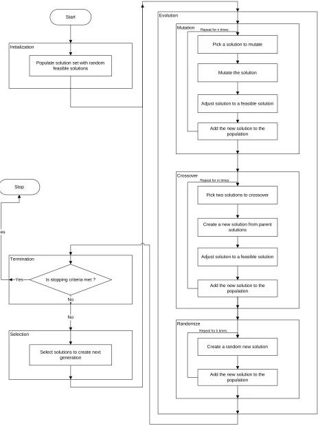
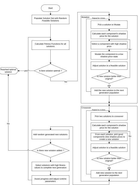
GA (Figure 3.1) is a reward based multi solution search algorithm. It is a branch of bio
inspired evolutionary algorithm (EA). Comparing to other single solution search algorithms such
as LP, k-opt algorithm, etc., there are multiple feasible solutions concurrently evolve toward the
best solution in the GA search process. The multiple generation search process ensures GA a
global search algorithm.
There are generally four major phases in the GA search process, initialization, evolution,
selection, and termination.
In the initialization phase, a startup solution population is created. Random generating
initial solutions are commonly used. All solutions in the population have to be feasible. The
population varies based on the problem to be solved and computing power available. It can be
range from 10s to hundreds or thousands. The initial solution shall spread out in the search space.
The more diverse the initial solutions, the better performance GA can achieve since it ensures
global search.
The evolution phase evolves current generation forward. The goal is to generate new
solutions based on current available solutions and hopefully the newly generated solutions are
better than current ones. There are two major methods to generate new solutions, binary operator
crossover and unary operator mutation.
The crossover operator mimics parents producing child in nature. Two solutions are
selected from the current generation’s solution pool and function as the “parents” to breed. Based
on problem domain, a breeding method is used to create the “child” solution. The child solution
participate the crossover operation. There are multiple ways to selection parents. The general
goal is to create a child solution that poses good characteristics of both parents and better than
both parents.
To generate a new solution, the unary mutation operator modifies the state(s) of one or a
small number of components of an existing solution. Most time, the newly generated solution is
much different than the original solution and may not even be a valid solution. Based on the
problem, the mutation operator may or may not generate a better solution. But it is a very
important operator that functions as an insurance of a global search. That is, it can bring search
to an area of search space that has not been visited before. It is especially important when GA
search stuck to a local optimal solution. In this case, mutation operator can lead search to another
area and effectively breaks the local trap. There are many methods to select which solution to
mutate and which component(s) to mutate.
Aside from mutation and crossover operators, several new solutions are randomly
generated in the evolution process in general as well. This is to further broaden the search space
and serves as an extra insurance of a global search.
After evolution phase generates enough new solutions, selection phase evaluates each
solution and select good solutions to create the next generation to continue evolution. It is also
called elitism. A fitness function is typically used to evaluate and compare solutions. Based on
different problem, the fitness function can be a simple linear function, a polynomial function, a
table look up, or a very complex optimization problem itself. As one of the stopping criteria in
general, this fitness function is also used to measure whether solutions meet predefined threshold
generation. Selecting good solutions can ensure search towards optimal solutions. Selecting
random solution ensures global search and avoid local optimal trap.
The termination phase evaluates the “goodness” of current solutions and decides whether
continue to evolve or stop. Since the optimal solution(s) is unknown for most problems,
predefined acceptable solution (defined by fitness function) can be used as one terminating
criterion. Maximum number of generations or maximum allowed time is also commonly used as
stopping criteria. Search progress is another barometer to evaluate GA’s searching process. It
can be measured by x progress in y generations. Combination of criteria or single criterion can
be used as the termination condition for search. After search stops, the best solution represents
the current search result. It can be optimal or near optimal based on the stopping criteria.
Random selection is used throughout the GA algorithm. It is used to select solution
participating mutation operation, crossover operation, or to participating next generation’s
evolution. There are two classic random selection method, roulette wheel and tournament.
In the roulette wheel selection, each candidate is assigned a probability of getting
selected. The sum of all candidates’ probabilities is equal to one. The probability of a solution is
related to its attribute(s). The fitness value can be a good choice. Obviously, solution with a large
probability has a better chance to be selected. The solution with small probability has a less
chance to be selected but still can be selected.
The tournament selection conducts one stage or multi stage tournament. It starts with
randomly organize candidates into groups. Within each group, a winning candidate is selected
based on probabilities assigned to the candidates. One way (Tournament Selection, 2010) is to
assign the best candidate a probability of p, the second best is assigned to p(1-p), the third best is
group are random grouped again for next stage tournament. The process repeats until desired
number of candidates are selected.
In summary, there are three GA operators that produce new solutions in the evolution
phase. They are mutation, crossover, and randomize. The mutation operator changes the state of
a component of a solution to move it closer to the optimal solution. The crossover operator tries
to create a better new solution from two existing solutions. Randomize operator introduces new
solutions. The initialization phase builds up the initial feasible solution pool to start off the
search process. The selection phase creates new generation of solutions to evolve forward from
current all available solutions. The termination phase ends the search process when predefined
Start
Stop
Yes
No
Evolution
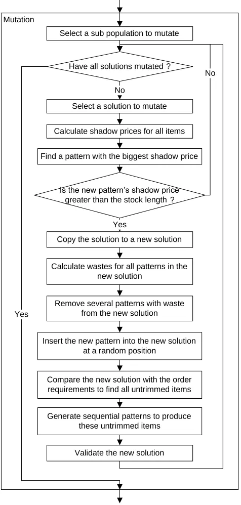
Mutation
Pick a solution to mutate
Mutate the solution
Adjust solution to a feasible solution
Add the new solution to the population Repeat for n times
Crossover
Pick two solutions to crossover
Create a new solution from parent solutions
Adjust solution to a feasible solution
Add the new solution to the population Repeat for m times
Randomize
Create a random new solution
Add the new solution to the population Repeat for k times Initialization
Populate solution set with random feasible solutions
Termination
Is stopping criteria met ?
Selection
Select solutions to create next generation Yes
[image:24.612.77.540.71.690.2]No
3.2 Opportunities
The main challenge that prevents GA’s further success is its performance issue. This
includes solution quality and search speed.
Randomness is used throughout the search process, such as building up the initial
solutions, choosing candidates to apply mutation or crossover operations, selecting solutions to
form next generations. It is also used in the GA operators. Mutation operator randomly selects a
component to mutate and mutate to a random state. Crossover operator randomly selects one or
many crossover point(s) to create new solution. All these randomness guides GA to randomly
select one or more solutions to evolve and move them to random state. The GA does not have a
uniformed search direction. It searches multiple directions in the same time. The selection
ensures GA search moving towards optimal solutions since better solutions are added into
generations to further evolve. It moves solution population closer to optimal solutions from
generation to generations in general.
Randomness is absolutely necessary to GA. It ensures GA a global search algorithm and
avoid local optimal trap. But it also slows down the search process since randomness can lead
search to all directions and cause many unnecessary searches. In the worst case, the randomness
can stall the search process and leads to sub optimal solutions, or visits all viable solutions.
There is a large amount of calculation in the GA search process. Within each generation
of search, each individual solution has to go through the process of inspection, evolution
operation, fitness value evaluation, and selection. It really takes much more time to process all
solutions in a generation than other single solution search algorithms such as heuristic, LP, etc.
Multiplying by many generations of evolution (synchronized or desynchronized), the total
complex GA search problems, where there are thousands of solutions in each generation and
search for thousands of generations, modern parallel computing techniques still cannot make
decisive impacts.
The other time consuming effort in the GA search process is the fitness function
calculation. For a simple problem, the fitness function can be a polynomial function which
calculation is rather straightforward and quick. However, the fitness function can be quite
complex in certain cases. For example, the fitness function can be a complicated matrix
operation or an optimization problem itself. Although GA poses little constraint on the
optimization problem, complex fitness function can add significant search time for complex
problem since the fitness function has to be calculated for all solutions.
Because GA takes long time to search, time constraint and/or generation constraint are
typically used as the stopping criteria. The idea is to get the best answer, which may not be the
optimal solution, within an acceptable time frame. This is the consequence from the GA’s slow
search speed. GA can stop searching prematurely and provide inferior result. The solution
CHAPTER 4 RELATED WORK
Since its introduction, much work has been dedicated to study GA’s performance.
Ishibuchi, Nojima, and Tsutomu (2006) studied the performance between single-objective GA
and objective GA. Using objective knapsack problem, they demonstrated that
multi-objective GA outperformed single-multi-objective GA for low count of multi-objectives problem. This is
because multi-objective GA can easily move away from local optimal. But when the objective
count increases, the multi-objective GA became less efficient. Simoncini, Collard, Verel, and
Clergue (2007) studied the impact of selection pressure to the performance of GA. They
confirmed that the selection pressure influence the GA performance using the anisotropic
selection and the stochastic tournament selection. More accurately compare and measure GA’s
performance has also been studied (Ang, Chong, & Li, 2002; Deng, Huang, & Tang, 2007).
Various innovations have been applied to GA to improve its performance. These
approaches can be roughly categorized as 1) transforming problem, 2) improving GA operators,
3) adding local search, 4) hybriding with other algorithms, 5) using parallel processing, and 6)
miscellaneous approaches.
4.1 Transforming Problem
Divide and conquer has long been used to solve complex problems. The idea is to divide
a large complex problem into smaller simpler problems. After solving each individual smaller
problem, results are combined to get the final solution. Zhang and Li (2007) applied the divide
and conquer theory into the EA. They decomposed the multi-objective optimization problem into
related scalar optimization sub problems. The scalar simpler sub problems are optimized
computation complexity is reduced greatly. Their experiments proved the new algorithm is very
efficient for 0-1 knapsack problems and continuous multi objective optimization problems.
Approximating is useful when certain tolerance is allowed in the value. This has
important practical values in many fields where tolerance is allowed or near optimal solution is
accepted. Paenke, Branke, and Jin (2006) and Regis and Shoemaker (2004) addressed the fitness
function’s computation complexity problem by substituting it with an approximate modal. Much
time can be saved by calculating simpler approximate fitness function. Their experiments proved
that the approximating is efficient and result qualities are acceptable.
The goal of problem transformation is to optimize one or more smaller simpler
problem(s) instead directly working on the more complex larger problems. Combining smaller
problems’ result, the final solution can be provided for the original problem. By optimizing less
computation intensive smaller simpler problems and reducing search space, the algorithm can
find optimal or near optimal solutions quicker.
4.2 Improving GA Operators
Syswerda (1991) introduced a new order crossover operation to preserver some order
information from both parents. It starts with randomly selecting n components from a parent.
Other non-selected components are passed to the child solution directly from the other parent.
They shall maintain their position like their parent. The selected n components are inserted into
the child solution based on their order from the first parent to complete the solution. For
example, there are two solutions S1= (A, B, C, D, E, F), S2= (B, F, E, D, C, A). If (B, D, E) is
randomly selected to preserve order from S1, the initial child solution from S2 using
non-selected components is C= (_, F, _, _, C, A). Adding non-selected components back in, the final child
Nagata and Kobayashi (1999) introduced an edge assembly crossover operator to
preserve the edge information from both parents. They started with building AB circles (parents
are named A, B) by selecting connecting edges from each parent alternately. The result is a set of
AB circles. A heuristic algorithm was used to connecting all AB circles into a final solution.
They applied the edge assembly crossover operator to the Traveling Salesman Problem (TSP)
and achieved good results.
Zhao, Dong, Li, and Yang (2008) added the pheromone concept from the Ant Colony
Optimization Algorithm (ACO) to enhance the crossover operation. They also used heuristic
method to solve the multiple- traveling salesman problem (mTSP). In their crossover operator,
the heuristic method use edge length and next city information. To decide which city to visit, the
child will look at both parents’ next visiting cities. If both cities from parents have already been
visited in the current solution, pheromone trail is used to select next visiting city.
The objective of improving GA operators is to pass some information from parent(s) to
the newly generated the child. There is no evaluation of whether the information passed actually
will move the search to the optimal solutions or not. It relies on the selection mechanism to
control the evolution towards the optimal since the selection will filter out inferior solutions.
This approach works in general at the cost of more calculations.
4.3 Adding Local Search
Noman and Iba (2008) designed a strategy adaptive hill-climbing crossover local search
(AHCXLS) in their EA. It used a simple hill-climbing algorithm to determine the search length
adaptively. It took feedback from search result to determine the search length. In their algorithm,
crossover is repeated until no better solution can be generated. They noticed, “there is no
crossover with one good candidate based on the fitness value and one randomly selected
solution.
Yang and Liu (2008) applied the local search to the solutions are have gone through
evolution operation. They searched the neighbor of the solution and replaced it with the best is
can find. Experiments shown the performance were much improved.
Tsai, Yang, and Kao (2002) added neighbor-join to the edge assembly crossover
operation. The neighbor-join operator will generate new solutions by using edges from other
solutions or generate new edges based on some heuristic information. The goal is to improve
solution quality.
Zhao, Dong, Li, and Yang (2008) used local search function to replace the mutation
operation. They used three types of local search to solve the mTSP problem. 1) Relocation
moves one city to a different location in the solution. 2) Exchange swaps positions of two cities.
3) 2-opt swaps end portions of two routes. They rotated these three local search operators. These
were used in addition to their improvement on the crossover operator described in the above
section.
Tseng and Chen (2009) used a two-phase genetic local search algorithm. The genetic
algorithm was used to search for promising areas in the first phase. The local search was used to
find the best solutions for the problem. Kaur and Murugappan (2008) used the nearest neighbor
as the local search algorithm to help populate initial solution pool for the GA. This way, the
algorithm starts from some better positions. Xuan and Li (2005) used local optimizer, 2-opt, to
optimize every solution after evolution. Zhang and Koduru (2005) used steepest ascent hill
climbing as the local search algorithm and also used blend crossover to improve GA’s
In this category, GA is improved by adding local search capability. The local search can
be used to enhance crossover operator, mutation operator, initial population build up, and
optimize resulting solutions from the evolution. Strictly speaking, adding local search to GA
results a hybrid algorithm. Since local search is used more often, I give it its own separate
category.
4.4 Hybriding with Other Algorithms
There are many hybrid algorithms that combine GA with many other search algorithms
such as Dantzig(1963) Simplex method, Nelder- Mead simplex method (Koduru, Dong, Das,
Welch, Roe, & Charbit, 2008; Nelder & Mead, 1965), etc. Most time, these additional search
algorithms perform local search while GA conducts global search. They are either used to
optimize solutions that have been applied GA operators (Koduru, Das, Welch, Roe, &
Lopez-Dee, 2005; Robin, Orzati, Moreno, Otte, & Bachtold, 2003) or used in conjunction with the GA
operators to improve its performance (Bersini, 2002; Tsutsui, Goldberg, & Sastry, 2001).
Although these are very important approaches, GA is the main algorithm and other algorithms
are simply assisting GA.
LP, on the other hand, has many ways to work with GA to create efficient hybrid
algorithms. Bredstrom, Carlsson, and Ronnqvist (2005) developed models and methods that
address the combined supply chain and production-planning problem. They developed a
mixed-integer-programming (MIP) model and solved the model using a heuristic solution based on
branch and bound. The model typically takes hours to solve. So, they created a GA algorithm to
solve the model. Each solution in the GA is a schedule and they used LP to make other decisions
for the schedule such as deciding shipping quantity in this case. To further speed up the LP
approaches had also been used by El-Araby, Yorino, and Zoka, (2005), El-Araby, Yorino, and
Sasaki (2002), and Leou (2008) where GAs were used to derive solution and successive linear
programming (SLP) and Simplex method were used to obtain the fitness values. In these
approaches, GA is the main driver of the program to conduct global search. LP is the help
algorithm that optimizes each solution and calculates fitness value.
LP has also been used to lead the search in the LP and GA hybrid algorithms. To design
the optimal fuel-cell-based energy network, Hayashi, Takeuchi, and Nozaki (2008) designed a
hybrid algorithm to account for the differences of equipment. Some energy equipment’s CO2
emission can be express in linear format and some cannot. LP cannot be used to precisely
optimize the overall modal. The hybrid algorithm used LP to design the optimal configuration
and evaluate the fitness function for equipment. GA takes the best LP configuration and
optimizes the overall installation while take in consideration of each equipment different CO2
emission characteristics. To design an optimal open magnetic resonance imaging magnet, Wang,
Xu, Dai, Zhao, Yan, and Kim (2009) first used LP to design the source current distribution and
used GA to optimize the section size of the cross-section of the coil. Pandey, Dong, Agrawal,
and Sivalingam (2007), Garg, Konugurthi, and Buyya (2009) designed similar hybrid algorithms
that use LP to generate initial solutions and have GA to fine-tune the solution. Although this kind
of LP/GA hybrid algorithm is straightforward conceptually, LP is used to create initial solutions
and GA searches for the final best solutions, it is a very efficient approach. By using LP
optimized solutions, GA is really starting the search from near optimal solutions. Thus, GA’s
search time is reduced significantly and can quickly reach optimal solutions. In certain cases, GA
Mantovani, Modesto, and Garcia (2001) combined GA and LP in a more efficient way.
They divided the reactive planning optimization problem into operating and planning sub
problems. The operating sub problem, a nonlinear and no convex problem, was solved by GA.
The planning sub problem, using real variables and linear problem, was solved by LP. Similar
approach was also used by Feng, Wang, and Li (2009).
LP and GA have different strengths. LP is very efficient in solving linear, non-integer
problems. GA has very little constraints on the objective function. LP can typically reach optimal
solution in a very short period of time. GA is slower. Integer LP is less efficient. Combining LP
and GA can typically reach optimal solutions for integer optimization problems quickly.
4.5 Using Parallel Processing
Parallel implementations of genetic algorithm (Alba & Tomassini, 2002; Liang, Chung,
Wong, & Duan, 2007; Massa et al., 2005; Ortiz-Garcia et al. 2009) have also been proposed and
experimented. There are a number of experiments, published papers with good results. With the
decreasing cost of computing resource, parallel algorithm became more and more appealing as
one of the methods to improve algorithm efficiency. There are many different ways to implement
parallel GA (PGA).
Hardware implementation of PGA refers to one kind of implementation in which partial
or complete algorithm (binary code) is encoded into the computer chips. The computer chips
become specialized for PGA purpose only. The code in the computer chips runs based on
computer clock cycles without software control. The common benefit of this implementation is
speed since there is no software involved. Jelodar, Kamal, Fakhraie, and Ahmadabadi (2006)
experimented a hardware based PGA using System-on-a-Programmable-Chip (SOPC). They
single processor genetic algorithm. b) Parallel GA using Master/Slave architecture c)
Coarse-grained PGA. To overcome the inflexibility of hardware based algorithm implementation, the
authors designed a mixed implementation approach: fitness evaluation in software and all other
GA/PGA elements in hardware. This approach allows complex fitness functions required by
difference category of problems. The experiments result showed the hardware based PGA is 50
times faster than software based PGA.
Scott, Samal, and Seth (1995) presented another working hardware based GA using
FPGA (field programmable gate array). There are two phases in the process. In phase I, user
enters the parameters of GA and the fitness function, system translate them into hardware image
and programs the FPGA. In phase II, upon front-end give a “go” signal, programmed FPGA run
the algorithms without any software interruption. When it’s finished, “done” signal was send to
the front-end. Finally, Front-end read the result. The authors’ experiment showed speedup factor
about 15.
Software implementation refers to PGA implementations where the algorithms run on
common computing resources without modify any underline hardware. Typically, there are a
group of general-purpose computers working together to implement PGA. There are four
models, 1) Global (master/slave) Model, 2) Fine-Grained Model, 3) Coarse-Grained Model, and
4) Hybrid Model.
Cantu-Paz (1997) published one of the frequent cited papers on the global model of PGA.
Based on the principle of divide and conquer, the classic global model uses one global
population and divides the task of evaluating fitness values of chromosomes among multiple
processors. In the model, there is a master processor that controls the whole process. The PGA
initializes the population, and send chromosomes to multiple processors (slaves) to evaluate
fitness value. After receive result from slave processors, master process performance all other
GA operators, such as selection, mutation, crossover, etc. With newly created population, master
processor sends chromosomes to slave processors to evaluate again. The process repeats until the
goal is satisfied.
Benkhider, Baba-Ali, and Drias (2007) proposed a generation less concept on GA and
two variation of general PGA model. The new GA mimic human population where there is
general concept of generation, no distinct clear-cut separation of generation and multiple
generations coexist in the same time. The new GA assigns each chromosome an effective start
and end time, i.e. a life span. Each chromosome would be replaced after it past its assigned end
time. In the meanwhile, new chromosomes were “born” and added to the population. They
proposed two new variations of global PGA. In the semi-asynchronous parallel approach, there
are two separate processes on the master processor. One is responsible for assigning
chromosomes to slave processors to evaluation and receiving results from them. The other one is
responsible of creating new chromosomes. The two processes works concurrently. Main
algorithm suspends when these two processes start to work and only resumes until both
processes complete their work. All GA operators are blocked when these two processes are
active. So, it is a semi asynchronous method. In the asynchronous master/slave approach, the two
processes do not block any other process. The other process is the main process. It’s the main
process that responsible for all GA operations (selection, mutation, crossover, etc.). It’s also
responsible for creating new chromosomes. Both processes work independent of each other and
The fine-grained architecture targets massive parallel computers. In this architecture,
there is only one population in the algorithm just like the global PGA architecture. There is no
master processor. There are a lot of inter-connected processors. They are connected in multiple
ways and most common is the grid structure. Each processor is responsible for a very small
population of chromosomes. Each processor executes a serial GA on its own population and
exchange result with neighbor processors. The ideal case is to have only one individual for every
processing element available. The efficient communication among interconnected node makes
the PGA very fast.
Lee, Park, and Kim (2000) proposed a binary tree structure to connect processors. Each
processor forwards its best individual to two next level processors and receives one from the top
processor. This is one-direction propagation. This slows down the chromosome migration rate.
And the tree structure is dynamic generated based on the position of the best chromosome. They
tested their proposal on CrayT3E with 64 processors and showed better performance. Li and
Kirley (2002) introduced a new concept “Percolation” into fine-grained PGA architecture. The
goal is to ease the selection pressure. They introduced a “seeding” method to the PGA in the
fine-grained architecture. When algorithm starts, a large number of random chosen processors
start with a chromosome and neighing processors forms demes. With the process evolving, new
processors become active and assigned with chromosomes. New processors join neighboring
demes to form larger demes. Eventually, all processors are active and forms one deme. This
process forms demes slowly and dynamically. There is no predefined size of deme. This
approach controls the rate of migration. Population diversity is maintained and high quality
Coarse-grained parallel genetic algorithm model uses multiple populations that evolve
separately and exchange individuals occasionally. It is also referred as multi-deme or distributed
PGAs. The basic idea of coarse-grained model is to divide the search space into several
sub-populations and assign each participating processor a sub-population. Each processor evolves its
population forward till goals are met. In the process, processors may exchange some good
chromosomes for speed up purpose. Although one processor may responsible of divide the initial
population to start the process and collect results at the end, there is no master processor that
controls each processor. Matsumura, Nakamura, Miyazato, Onaga, and Okech (1997)
experimented on ring, torus, and hypercube topologies. They concluded that Ring topology and
emigrant method provide the best result.
In an attempt to use cycle-steal method to harvest the computing power that scatted over
the Internet, Berntsson and Tang (2003) studied the coarse-grained architecture of PGA. They
conducted multiple experiments with different topologies, different migration rate, different
migration intervals and different failure scenarios. They used 4 faster processors and 4 slow
processors to build a heterogeneous computing network. To work with Internet's latency and
bandwidth problems, they concluded that a small migration rate with long migration intervals
and a fully connected topology would be the best choice.
The hybrid model, a combination of different model of PGA, is a new model that results
in algorithms that have the benefits of different PGA models. The new model may show better
performance than any of the models alone. The combined model is more complex and difficult to
program. But they do not introduce new analytic problems, and it can be useful when working
with complex applications. The combination can varies, such as coarse-grained with global
model, etc. The combination does not limit to within the PGA models. New models can include
other optimization algorithms, such as LP, nearest neighbor algorithm, etc.
Lee, Park, & Kim (2001) proposed a hybrid PGA architecture to address two issues, to
connect large amount of processors in the PGA calculation and to control the migration speed to
achieve better result (alleviating super chromosome dominating solution space issue). High-level
processors used coarse-grained model to connect to each other. Chromosome migration rate is
low. Lower level processors using fine-grained PGA model and the migration rate is high. The
fine-grained PGA used binary tree model to organize. The tree is built dynamically based on the
location of the best solution and communication is one directional, from top to bottom only. The
tree structure decides the processor to receive chromosome from or processors to send to. To
further minimize the dominating solution issue, limits are put on migration policy.
Zhao, Man, Wan, & Bi (2008) introduced a multi-agent hybrid parallel genetic algorithm.
They combined global PGA model with coarse-grained PGA model. In the new model, there are
master agents and slave agents. Each master agent (M-agent) is in charge of several slave agents
(A-agent) to form a global master slave PGA model. The M-agent responsible for the evolution
process and A-agent helps with the parallel calculation. Several M-agents connect to each other
to form a coarse grained PGA model.
Genetic algorithm is a good candidate to be parallelized. The simple algorithm made it
easy to be implemented and tested. It’s a fault tolerant algorithm since its population can be
large. PGA can make GA fast and efficient. A good design of PGA shall have following
attributes. It fully utilizes available computing resources. Communication is efficient and simple.
Migration policy ensures a diverse sub populations and fast to converge to the global optimal
4.6 Miscellaneous Approaches
Yuen, S.Y., & Chow (2009) used a binary space partitioning tree to archive the solutions
that GA has visited. Based on the binary tree, they designed a novel adaptive mutation operator.
The mutation operation is replaced by searching the tree. They start with locating the solution to
be mutated in the tree. Then, they find the nearest neighbor-unvisited subspace of the solution
and random select one as the mutation result. If all nearest neighbor solution has been visited,
backtrack to the parent and repeat the process. In the meanwhile, fully visited sub tree can be
trimmed from the tree. The algorithm visits a nearest unvisited neighbor subspace and randomly
finds an unvisited solution in it. They named the algorithm as “A Genetic Algorithm That
Adaptively Mutates and Never Revisits”.
Throughout GA’s search process, random number is used frequently. A random number
generator is typically used. It is an algorithm that generates long sequences of random numbers
based on the initial value. These random numbers are not true random since they are predictable
and repeatable. The same sequence of numbers can be reproduced by the same algorithm using
the same initial value. They are pseudo random numbers. Caponetto, Fortuna, Fazzino, and
Xibilia (2003) replaced random number with chaotic time series sequences in the algorithm.
Simulation results and their statistical analysis using the t-test method showed distinct
improvement from using chaotic sequences for the tested problems.
Singh, Isaacs, Nguyen, Ray, Yao (2008) and Singh, Isaacs, Ray, Smith (2008) proposed
an Infeasibility Driven Evolutionary Algorithm (IDEA). The algorithm ranks solutions based on
the original objectives (fitness function) along with additional objectives that reflects constraint
several infeasible solutions in the generation to maintain the diversity of solution pool. The
experiments result showed a fast convergence to optimal solutions.
There are many other development that enhancing the GA’s performance such as
cooperative co-evolution (Adra, Dodd, Griffin, & Fleming, 2009), convergence accelerator (Tan,
Teo, & Lau, 2007), etc. Due to the fact that GA is a straight forward global search algorithm and
has demonstrated its effectiveness in many applications, more and more researchers are spending
more time enhancing it with many other algorithms or methods. In the meanwhile, GA is
CHAPTER 5 DUALITY AND SHADOW PRICE in LINEAR PROGRAMMING
5.1 Definition
Dantzig (1963) stated, “The linear programming model needs an approach to finding a
solution to a group of simultaneous linear equations and linear inequalities that minimize a linear
form.” LP is the algorithm to search for an optimal value for a linear objective function that
satisfies linear equations and linear inequalities.
Kolman and Beck (1980) defined the standard form for LP as,
For values of x1,x2,,xn which will maximize
n nx c x c x c
z 1 1 2 2 (5.1)
Subject to the constraints
1 1
2 12 1
11x a x a x b
a n n
2 2
2 22 1
21x a x a x b
a n n (5.2)
m n n m m
m x a x a x b
a 1 1 2 2 1
xj 0,j1,2,n
More conveniently, we can use a matrix notation. Let
mn m m n n a a a a a a a a a A 2 1 2 22 21 1 12 11 , m b b b b 2 1 , n x x x x 2 1 , n c c c c 2 1 (5.3)
A LP standard form can be rewritten as
Maximize zcTx (5.4)
Subject to Axb
The Duality Theorem states that there is an equivalent LP problem for every LP problem.
One is called the primal problem and the other is called the dual problem. Dantzig (1963)
proved the duality theorem. The dual problem for the above standard form is given below.
For values of y1,y2,,ym which will minimize
m my b y b y b
z' 1 1 2 2 (5.5)
Subject to the constraints
1 1
2 21 1
11y a y a y c
a m m
2 2
2 22 1
12y a y a y c
a m m (5.6)
n m mn n
ny a y a y c
a1 1 2 2
yj 0,j1,2,m
The matrix representation is
Minimize z bTy
' (5.7)
Subject to ATyc
y0
where m y y y y 2 1
The Duality Theorem also states that if the primal problem has an optimal solution (x0)
and the dual problem has an optimal solution (y0), then
zcTx0 z'bTy0 (5.8)
Solving one LP problem is equivalent to solving its dual problem. Kolman and Beck
(1980) described the shadow prices as,
j m
i i
ijy c
a
1
(5.9)
The coefficient aij represents the amount ofinput i per unit of output j, and the right-hand
side is the value per unit of output j. This means that the units of the dual variable yi are the
“value per unit of input i”; the dual variables act as prices, costs, or values of one unit of each of
the inputs. They are referred as dual prices, fictitious prices, shadow prices, etc.
In general term, shadow price is the contribution to the objective function that can be
made by relaxing a constraint by one unit. Different constraints have different shadow prices,
and every constraint has a shadow price. Each constraint’s shadow price changes along with the
algorithm searching progress.
5.2 Shadow Prices in Linear Programming
LP has been used widely in various industrial fields. With a concrete mathematical
model, it provides direct relationships among profit and constraints, output and constraints, other
goals and constraints, etc. The linear models can be solved efficiently. Dantzig’s (1963) Simplex
method is one of them.
LP requires all constraints and all possible activities that meet the constraints listed in the
tabular format. This is not a problem when the number of possible activities is small, such as
maximizing profit for a small manufacturer. Constraints are material or labor and the objective
function is defined as profit. It is rather straightforward to define the linear constraints, construct
the linear objective function and search for optimal solutions for this category of problems.
It gets complicated where the number of possible activities is very large, such as the
typical scheduling problems and the cutting stock problems. For these problems, there are a very
constraints. For a good-sized airline, there are complex flight schedules, a large number of
routes, and many flight crews. Various goals can be optimized, such as finding the minimal
number of crews needed to cover all flights while satisfying airline regulations, creating the crew
schedules while balancing flight hours among crews, creating crew schedules to minimize cost,
etc.. There are many possible combination of assigning crews to flights. This is an activity
number explosion problem. For each activity, a separate variable need to be defined for the
objective function and a separate column in the constraint matrix needs to be created in LP. This
creates a very large number of variables and constraint columns. It is almost impossible to create
a LP model with all possible activity combinations listed and constraints defined for this kind of
problems. Solving these huge problems will be very time consuming and inefficient.
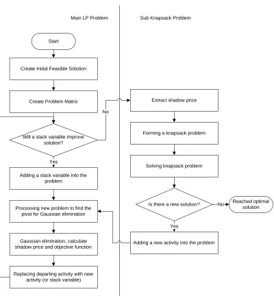
Gilmore and Gomory (1961, 1963, 1965, & 1966) developed a dynamic column
generation algorithm to deal with this kind of combination explosion LP problem. They
demonstrated their algorithm using the complex cutting stock problem. Figure 5.2.1 is the high
level flow chart of their algorithm.
The Gilmore and Gomory’s breakthrough is separating the large problem into two
smaller problems. The objective for the main LP problem (Figure 5.1 Main LP Problem) is to
find the best solution using current available activities. The sub problem (Figure 5.1 Sub
Knapsack Problem) is a knapsack problem. The solution from the main problem provides the
coefficients for the sub problem’s constraints. The solution from the sub problem is a newer and
better activity that can be utilized by the main algorithm. The process alternates between solving
the main and the sub problem until there is no better solution that can be generated by the sub
The coefficients supplied by the main algorithm to the sub algorithm are the shadow
prices (dual prices). The knapsack sub problem is constructed using these shadow prices. For
different iterations, the main algorithm provides the sub algorithm with different shadow prices
based on the current best solution. That is, the shadow prices change along with the algorithm’s
searching process.
Create Initial Feasible Solution
Create Problem Matrix
Will a slack variable improve solution?
Adding a slack variable into the problem
Processing new problem to find the pivot for Gaussian elimination
Gaussian elimination, calculate shadow price and objective function
Replacing departing activity with new activity (or slack variable)
Extract shadow price
Forming a knapsack problem
Solving knapsack problem
Adding a new activity into the problem
Is there a new solution? Reached optimal solution Start
Yes
No
Yes
[image:45.612.126.526.231.663.2]No Main LP Problem Sub Knapsack Problem
CHAPTER 6 SHADOW PRICE GUIDED GENETIC ALGODITHM
6.1 The Concept
We have developed a secondary measurement (Shen & Zhang, 2011-1) for solutions in
the GA using the shadow price concept. We use the shadow prices to measure components in a
solution as a complement measurement to the fitness function. Thus, we establish a
two-measurement system: fitness values are used to evaluate overall solutions and shadow prices are
used to evaluate components.
Using GA to solve a problem P, there is a current solution population R that has n
solutions and each solution has m components. The jth solution is defined as
) , , ,
( 1j 2j mj
j a a a
S where aij represents ith component in jth solution. Then, the current
solution space is ( 1 , 2, , T)
n T T S S S
R . Furthermore, we can define a correspondent LP problem
as: mn m m n n a a a a a a a a a A 2 1 2 22 21 1 12 11 , m b b b b 2 1 , n x x x x 2 1 , n c c c c 2 1 (6.1)
Optimize zcTx (6.2)
Subject to Ax()()()b
x is binary variable 0 or 1
and
n i i x 1 1ci is the fitness value of each solution. The objective is to find the solution with the best fitness
This approach cannot deal with the combination explosion situation. We cannot possibly
enumerate all feasible combinations in the A matrix. For example, there are over 3 million
possible combinations for a merely 10 cities’ traveling salesman problem. Secondly, we cannot
always define the b vector. We probably can create the b vector for the value-combination
problems. But for the position-combination problems, such as the traveling salesman problem, it
is very difficult to find the meaning of the b vector or define the relationship between Ax and b.
The key of our approach is to use shadow price to compare components to further
improve EA. In EA, we define the shadow price as the relative potential improvement to the
solution’s (chromosome) fitness value with a change of a component (gene). It’s a relative
potential improvement since the concept is defined on a single component and a component
change may force other components’ change to maintain solution feasibility. The improvement
may or may not be realizable. A change of component states the fact that component change can
be a value change or a position change.
Shadow prices can take on different meanings or values for different problems. In the
traveling salesman problem, it can simply be the possible distance reduction from changing the
next visiting city. But the definition has to be clear and comparable among components.
The fitness value represents the current solution’s position in the search space. The
shadow prices represent potential improvements and directions to evolve. The shadow prices are
only meaningful in the process of evolution. They shall be used for selecting components to
evolve and for setting directions for evolution operators. While choosing candidate solutions that
are close to the optimal to further evolve, we shall also include solutions with bigger potential
improvements. The potential improvement of a solution can be defined as the sum of all