www. ijraset.com
Volume 2 Issue IX, September 2014
ISSN: 2321-9653
International Journal for Research in Applied Science & Engineering
Technology(IJRASET)
Analysis of Spatial domain and Frequency
domain Techniques for Car plate detection
G.P.S.Manideep
1, Prof.G. K. Rajini
2, A.Sharmila
3School of Electrical Engineering, VIT University Vellore - 632014, India
Abstract :In last couple of decades, the number of automobiles has increased drastically. With this increase, it is difficult to keep track of each automobile for purpose of law enforcement and traffic management. License Plate Recognition is used increasingly nowadays for automatic toll collection, maintaining traffic activities and law enforcement. Many techniques have been proposed for plate detection, each having its own advantages and disadvantages. The basic step in License Plate Detection is localization of number plate. The approaches mentioned in this work are a Spatial domain(Histogram Based Approach(HBA)) and transform domain(Steerable wavelet) for car license plate detection analysis is done for both approaches by performance measures like Peak signal to noise ratio(PSNR),Mean square error(MSE) and success ratio, consumption time. The transform domain technique using steerable wavelets seems to be promising for this application.
I. INTRODUCTION
With increasing number of automobiles on roads, it is difficult to manually enforce laws and traffic rules for smooth traffic process. Toll-booths are constructed on freeways and parking structures, where the car has to stop to pay the toll or parking fees. Also, Traffic Management systems are installed on freeways to check for automobiles moving at speeds not permitted by law. In order to automate these processes and make them more effective, a system is required to easily identify an individual automobile. The important question here is how to identify a particular automobile? The obvious answer to this question is by
using the automobile’s number plate. Automobiles in each country have a unique license number, which is written on its license
plate. This number distinguishes one automobile from the other, which is useful especially when both are of same make and model. An automated system can be implemented to identify the license plate of an automobile and extract the characters from the region containing a license plate. The license plate number can be used to retrieve more information about the automobile and its owner, which can be used for further processing. Such an automated system should be small in size, portable and be able to process data at sufficient rate. Various license plate detection algorithms have been developed in past few years. Each of these algorithms has their own advantages and disadvantages. As multiple detections are available for single license plate, post
–processing methods are applied to merge all detected regions. In addition, trackers are used to limit the search region to certain areas in an image. Kwasnickaet al. [1] suggests a different approach of detection using binarization and elimination of unnecessary regions from an image. In this approach, initial image processing and binarization of an image is carried out based on the contrast between characters and background in license plate. After binarizing the image, it is divided into different black and white regions. These regions are passed through elimination stage to get the final region having most probability of containing a number plate.
II. EDGE DETECTION
Edges characterize object boundaries and are therefore useful for segmentation, registration and identification of the objects in scenes. Edge points can be thought of as pixel locations of abrupt gray-level change [12]. For example, it is reasonable to define edge points in binary images as black pixels with at least one white nearest neighbour , that is, pixel locations (m,n) such that u(m, n)=0 and g(m,n)=1, where
g(m, n)≜[u(m, n)u(m ± 1, n)]OR[u(m, n)u(m, n± 1)]…...Eq2.1
III. SPATIAL DOMAIN APPROACH
www. ijraset.com
Volume 2 Issue IX, September 2014
ISSN: 2321-9653
International Journal for Research in Applied Science & Engineering
Technology(IJRASET)
Page 485
g(xi) =∑jαjxj …..Eq3.1IV. TRANSFORM DOMAIN APPROACH
The selection of the transform for the first implementation is governed by prior knowledge about image spectra in the transform domain, Accuracy of empirical spectrum estimation, Transform energy compaction capability, and computational complexity of the filtering in the transform domain. Some of these feasible transforms are DFT, DCT, DST, Haar , Walsh, Wavelets .
A. Wavelet Transform
The fundamental idea of wavelet transforms is that the transformation should allow only changes in time extension, but not shape. This is affected by choosing suitable basis functions that allow for this. Changes in the time extension are expected to conform to the corresponding analysis frequency of the basis Multi resolution features time frequency domain information can be obtained simultaneously.
1) DWT
The DWT of a signal is calculated by passing it through a series of filters. First the samples are passed through a low pass filter with impulse response resulting in a convolution of the two:
[ ] = ( ∗ )[ ] = ∑∞ [ ] [ − ]
∞ ……...Eq4.1
The signal is also decomposed simultaneously using a high pass filter h. The outputs giving the detail coefficients (from the high-pass filter) and approximation coefficients (from the low pass). It is important that the two filters are related to each other and they are known as a quadrature mirror filter.
However, since half the frequencies of the signal have now been removed, half the samples can be discarded according to
Nyquist’s rule. The filter outputs are then subsampled by 2 (Mallat' s and the common notation is the opposite, g- high pass and
h- low pass):
[ ] = ∑∞ [ ]ℎ[2 − ]
∞ ……….Eq4.2
[ ] = ∑∞ [ ] [2 − ]
∞ ……….Eq4.3
2) CWT
Continuous wavelet transform (CWT) is used to divide a continuous-time function into wavelets. Unlike Fourier transform, the continuous wavelet transform possesses the ability to construct a time-frequency representation of a signal that offers very good time and frequency localization. The continuous wavelet transform of a continuous, square-integral function.
( , ) = | |∫∞∞ ( ) ……Eq4.4
B. Steerable wavelets
Oriented filters are used in many vision and image processing tasks, such as texture analysis, edge detection, image data compression, and motion analysis and image enhancement. In many of these tasks, it is useful to apply filters of arbitrary orientation under adaption control, and to examine the filter output as a function of both orientation and phase. There are techniques that allow synthesis of a filter at arbitrary orientation and phase, and will develop methods to analyse the filter outputs. We will also describe efficient architectures for such processing, develop flexible design methods for filter in two and three dimensions, and apply the filters to several tasks in image analysis. One approach to finding the response of a filter at many orientations is to apply many versions of the same filter each different from the others by some small rotation in angle. A more efficient approach is to apply a few filters corresponding to a few angles and interpolate between the responses. With the correct filter set and the correct interpolation rule, it is possible to determine the response of a filter of arbitrary orientation without explicitly applying that filter. We will show that two and three dimensional functions are steerable, and will show how many basis filters are needed to steer a given filter.
C. Steerable Wavelet Properties
By using the fact that the polar representation of the Fourier transform of Rnψ(x) ise θh(ω)we can readily show that the
Fourier transform of a generic steerable wavelet is polar-separable
www. ijraset.com
Volume 2 Issue IX, September 2014
ISSN: 2321-9653
International Journal for Research in Applied Science & Engineering
Technology(IJRASET)
Page 485
g(xi) =∑jαjxj …..Eq3.1IV. TRANSFORM DOMAIN APPROACH
The selection of the transform for the first implementation is governed by prior knowledge about image spectra in the transform domain, Accuracy of empirical spectrum estimation, Transform energy compaction capability, and computational complexity of the filtering in the transform domain. Some of these feasible transforms are DFT, DCT, DST, Haar , Walsh, Wavelets .
A. Wavelet Transform
The fundamental idea of wavelet transforms is that the transformation should allow only changes in time extension, but not shape. This is affected by choosing suitable basis functions that allow for this. Changes in the time extension are expected to conform to the corresponding analysis frequency of the basis Multi resolution features time frequency domain information can be obtained simultaneously.
1) DWT
The DWT of a signal is calculated by passing it through a series of filters. First the samples are passed through a low pass filter with impulse response resulting in a convolution of the two:
[ ] = ( ∗ )[ ] = ∑∞ [ ] [ − ]
∞ ……...Eq4.1
The signal is also decomposed simultaneously using a high pass filter h. The outputs giving the detail coefficients (from the high-pass filter) and approximation coefficients (from the low pass). It is important that the two filters are related to each other and they are known as a quadrature mirror filter.
However, since half the frequencies of the signal have now been removed, half the samples can be discarded according to
Nyquist’s rule. The filter outputs are then subsampled by 2 (Mallat' s and the common notation is the opposite, g- high pass and
h- low pass):
[ ] = ∑∞ [ ]ℎ[2 − ]
∞ ……….Eq4.2
[ ] = ∑∞ [ ] [2 − ]
∞ ……….Eq4.3
2) CWT
Continuous wavelet transform (CWT) is used to divide a continuous-time function into wavelets. Unlike Fourier transform, the continuous wavelet transform possesses the ability to construct a time-frequency representation of a signal that offers very good time and frequency localization. The continuous wavelet transform of a continuous, square-integral function.
( , ) = | |∫∞∞ ( ) ……Eq4.4
B. Steerable wavelets
Oriented filters are used in many vision and image processing tasks, such as texture analysis, edge detection, image data compression, and motion analysis and image enhancement. In many of these tasks, it is useful to apply filters of arbitrary orientation under adaption control, and to examine the filter output as a function of both orientation and phase. There are techniques that allow synthesis of a filter at arbitrary orientation and phase, and will develop methods to analyse the filter outputs. We will also describe efficient architectures for such processing, develop flexible design methods for filter in two and three dimensions, and apply the filters to several tasks in image analysis. One approach to finding the response of a filter at many orientations is to apply many versions of the same filter each different from the others by some small rotation in angle. A more efficient approach is to apply a few filters corresponding to a few angles and interpolate between the responses. With the correct filter set and the correct interpolation rule, it is possible to determine the response of a filter of arbitrary orientation without explicitly applying that filter. We will show that two and three dimensional functions are steerable, and will show how many basis filters are needed to steer a given filter.
C. Steerable Wavelet Properties
By using the fact that the polar representation of the Fourier transform of Rnψ(x) ise θh(ω)we can readily show that the
www. ijraset.com
Volume 2 Issue IX, September 2014
ISSN: 2321-9653
International Journal for Research in Applied Science & Engineering
Technology(IJRASET)
ψ ( ) = ∑ u R ψ(x) ↔ψ (ω) = h(ω)u(θ)...4.5
whereu(θ) = ∑ u e θis 2π-periodic. Conversely, we have the guarantee that the proposedrepresentation provides a full
parameterization of the wavelets whose Fourier transformis polar-separable because the complex exponentials {e θ}n∈Z form
a basis ofL ([−π, π]).The steerable waveletψGen(x) is real-valued if and only if its Fourier transform is Hermitian-symmetric (i.e.,ΨGen(−ω) =ΨGen(ω)). Since the real term h(ω) can be factored out,this gets translated into the angular conditionu(θ+
π) =u(θ). Additionally, we can imposesymmetry by considering Fourier series with even or odd harmonic terms.
V. MATLAB SIMULATION
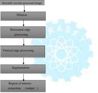
The Flow chart used for license plate detection using spatial domain approach is shown in Fig5.1
Input image
Fig.5.1 Flowchart of license plate detection using spatial domain approach
A. Convert a Coloured Image into Gray Image
Colour to gray
conversion
Dilation
Horizontal edge
processing
Vertical edge processing
Segmentation
Region of interest
extraction (output)
www. ijraset.com
Volume 2 Issue IX, September 2014
ISSN: 2321-9653
International Journal for Research in Applied Science & Engineering
Technology(IJRASET)
ψ ( ) = ∑ u R ψ(x) ↔ψ (ω) = h(ω)u(θ)...4.5
whereu(θ) = ∑ u e θis 2π-periodic. Conversely, we have the guarantee that the proposedrepresentation provides a full
parameterization of the wavelets whose Fourier transformis polar-separable because the complex exponentials {e θ}n∈Z form
a basis ofL ([−π, π]).The steerable waveletψGen(x) is real-valued if and only if its Fourier transform is Hermitian-symmetric (i.e.,ΨGen(−ω) =ΨGen(ω)). Since the real term h(ω) can be factored out,this gets translated into the angular conditionu(θ+
π) =u(θ). Additionally, we can imposesymmetry by considering Fourier series with even or odd harmonic terms.
V. MATLAB SIMULATION
The Flow chart used for license plate detection using spatial domain approach is shown in Fig5.1
Input image
Fig.5.1 Flowchart of license plate detection using spatial domain approach
A. Convert a Coloured Image into Gray Image
Colour to gray
conversion
Dilation
Horizontal edge
processing
Vertical edge processing
Segmentation
www. ijraset.com
Volume 2 Issue IX, September 2014
ISSN: 2321-9653
International Journal for Research in Applied Science & Engineering
Technology(IJRASET)
Page 487
Fig 5.2 Original image Fig 5.3 Gray image
The algorithm described here is independent of the type of colours in image and relies mainly on the gray level of an image for processing and extracting the required information. Colour components like Red, Green and Blue value are not used throughout this algorithm. So, if the input image is a coloured image represented by 3-dimensional array in MATLAB, it is converted to a 2-dimensional gray image before further processing. The sample of original input image is shown in Fig 5.2 and a gray image is shown in Fig 5.3
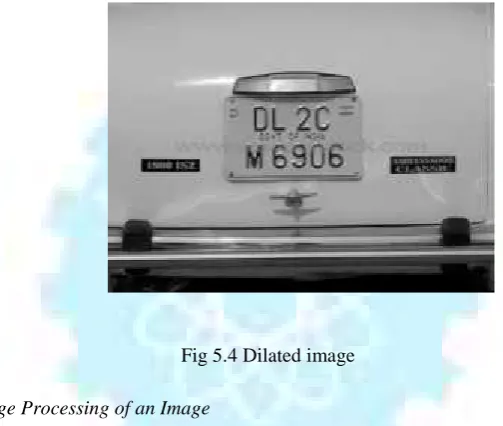
B. Dilate an Image
[image:5.595.164.416.294.507.2]Dilation is a process of improving a given image by filling holes in an image, sharpen the edges of objects in an image, and join the broken lines and increase the brightness of an image. Using dilation, the noise with-in an image can also be removed. By making the edges sharper, the difference of gray value between neighbouring pixels at the edge of an object can be increased which enhances the edge detection. In Number Plate Detection, the image of a car plate may not always contain the same brightness and shades. Therefore, the given image has to be converted from RGB to gray form. The process of dilation will help to nullify such losses. The image below shows such figure in Fig 5.4
Fig 5.4 Dilated image
C. Horizontal and Vertical Edge Processing of an Image
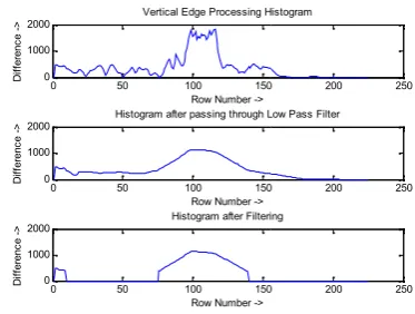
Histogram is a graph representing the values of a variable quantity over a given range. These histograms represent the sum of differences of gray values between neighbouring pixels of an image, column-wise and row-wise. In the above step, first the horizontal histogram is calculated. To find a horizontal histogram, the algorithm traverses through each column of an image. In each column, the algorithm starts with the second pixel from the top. The difference between second and first pixel is calculated. If the difference exceeds certain threshold, it is added to total sum of differences. Then, algorithm will move downwards to calculate the difference between the third and second pixels. So on, it moves until the end of a column and calculate the total sum of differences between neighbouring pixels. At the end, an array containing the column-wise sum is created. The same process is carried out to find the vertical histogram. In this case, rows are processed instead of columns.
D. Passing Histograms through a Low Pass Digital Filter
Referring to the figures shown below, one can see that the histogram values changes drastically between consecutive columns and rows. Therefore, to prevent loss of important information in upcoming steps, it is advisable to smooth out such drastic changes in values of histogram. For the same, the histogram is passed through a low-pass digital filter. While performing this step, each histogram value is averaged out considering the values on it right-hand side and left-hand side. This step is performed on both the horizontal histogram as well as the vertical histogram. Below are the figures showing the histogram before passing through a low-pass digital filter and after passing through a low-pass digital filter in Fig 5.5 and Fig 5.6 respectively.
www. ijraset.com
Volume 2 Issue IX, September 2014
ISSN: 2321-9653
International Journal for Research in Applied Science & Engineering
Technology(IJRASET)
Page 487
Fig 5.2 Original image Fig 5.3 Gray image
The algorithm described here is independent of the type of colours in image and relies mainly on the gray level of an image for processing and extracting the required information. Colour components like Red, Green and Blue value are not used throughout this algorithm. So, if the input image is a coloured image represented by 3-dimensional array in MATLAB, it is converted to a 2-dimensional gray image before further processing. The sample of original input image is shown in Fig 5.2 and a gray image is shown in Fig 5.3
B. Dilate an Image
Dilation is a process of improving a given image by filling holes in an image, sharpen the edges of objects in an image, and join the broken lines and increase the brightness of an image. Using dilation, the noise with-in an image can also be removed. By making the edges sharper, the difference of gray value between neighbouring pixels at the edge of an object can be increased which enhances the edge detection. In Number Plate Detection, the image of a car plate may not always contain the same brightness and shades. Therefore, the given image has to be converted from RGB to gray form. The process of dilation will help to nullify such losses. The image below shows such figure in Fig 5.4
Fig 5.4 Dilated image
C. Horizontal and Vertical Edge Processing of an Image
Histogram is a graph representing the values of a variable quantity over a given range. These histograms represent the sum of differences of gray values between neighbouring pixels of an image, column-wise and row-wise. In the above step, first the horizontal histogram is calculated. To find a horizontal histogram, the algorithm traverses through each column of an image. In each column, the algorithm starts with the second pixel from the top. The difference between second and first pixel is calculated. If the difference exceeds certain threshold, it is added to total sum of differences. Then, algorithm will move downwards to calculate the difference between the third and second pixels. So on, it moves until the end of a column and calculate the total sum of differences between neighbouring pixels. At the end, an array containing the column-wise sum is created. The same process is carried out to find the vertical histogram. In this case, rows are processed instead of columns.
D. Passing Histograms through a Low Pass Digital Filter
www. ijraset.com
Volume 2 Issue IX, September 2014
ISSN: 2321-9653
[image:6.595.94.292.81.237.2] [image:6.595.308.495.91.232.2]International Journal for Research in Applied Science & Engineering
Technology(IJRASET)
Fig 5.5 Horizontal image processing Fig 5.6 Vertical image processing
E. Filtering out Unwanted Regions in an Image
Once the histograms are passed through a low-pass digital filter, a filter is applied to remove unwanted areas from an image. In this case, the unwanted areas are the rows and columns with low histogram values. A low histogram value indicates that the part of image contains very little variations among neighbouring pixels. Since a region with a license plate contains a plain background with alphanumeric characters in it, the difference in the neighbouring pixels, especially at the edges of characters and number plate, will be very high. This results in a high histogram value for such part of an image.
Therefore, a region with probable license plate has a high horizontal and vertical histogram values. Areas with less value are thus not required anymore. Such areas are removed from an image by applying a dynamic threshold. In this algorithm, the dynamic threshold is equal to the average value of a histogram. Both horizontal and vertical histograms are passed through a filter with this dynamic threshold. The output of this process is histogram showing regions having high probability of containing a number plate. The filtered histograms are shown in fig 5.5 and 5.6
F. Segmentation
[image:6.595.49.554.378.682.2]The next step is to find all the regions in an image that has high probability of containing a license plate using segmentation process. Co-ordinates of all such probable regions are stored
Fig 5.7 Segmentation Fig 5.8 output image
in an array. The Segmented image displaying these regions is shown in Fig 5.7.
0 50 100 150 200 250 300 350 400 450 500
0 5000
10000 Horizontal Edge Processing Histogram
Column Number ->
D iff er en ce ->
0 50 100 150 200 250 300 350 400 450 500
0
5000 Histogram after passing through Low Pass Filter
Column Number ->
D iff er en ce ->
0 50 100 150 200 250 300 350 400 450 500
0
5000 Histogram after Filtering
Column Number ->
D iff er en ce ->
www. ijraset.com
Volume 2 Issue IX, September 2014
ISSN: 2321-9653
International Journal for Research in Applied Science & Engineering
Technology(IJRASET)
Fig 5.5 Horizontal image processing Fig 5.6 Vertical image processing
E. Filtering out Unwanted Regions in an Image
Once the histograms are passed through a low-pass digital filter, a filter is applied to remove unwanted areas from an image. In this case, the unwanted areas are the rows and columns with low histogram values. A low histogram value indicates that the part of image contains very little variations among neighbouring pixels. Since a region with a license plate contains a plain background with alphanumeric characters in it, the difference in the neighbouring pixels, especially at the edges of characters and number plate, will be very high. This results in a high histogram value for such part of an image.
Therefore, a region with probable license plate has a high horizontal and vertical histogram values. Areas with less value are thus not required anymore. Such areas are removed from an image by applying a dynamic threshold. In this algorithm, the dynamic threshold is equal to the average value of a histogram. Both horizontal and vertical histograms are passed through a filter with this dynamic threshold. The output of this process is histogram showing regions having high probability of containing a number plate. The filtered histograms are shown in fig 5.5 and 5.6
F. Segmentation
The next step is to find all the regions in an image that has high probability of containing a license plate using segmentation process. Co-ordinates of all such probable regions are stored
Fig 5.7 Segmentation Fig 5.8 output image
in an array. The Segmented image displaying these regions is shown in Fig 5.7.
0 50 100 150 200 250 300 350 400 450 500
0 5000
10000 Horizontal Edge Processing Histogram
Column Number ->
D iff er en ce ->
0 50 100 150 200 250 300 350 400 450 500
0
5000 Histogram after passing through Low Pass Filter
Column Number ->
D iff er en ce ->
0 50 100 150 200 250 300 350 400 450 500
0
5000 Histogram after Filtering
Column Number ->
D iff er en ce ->
0 50 100 150 200 250
0 1000
2000 Vertical Edge Processing Histogram
Row Number ->
D iff er en ce ->
0 50 100 150 200 250
0 1000
2000 Histogram after passing through Low Pass Filter
Row Number ->
D iff er en ce ->
0 50 100 150 200 250
0 1000
2000 Histogram after Filtering
Row Number ->
D iff er en ce ->
www. ijraset.com
Volume 2 Issue IX, September 2014
ISSN: 2321-9653
International Journal for Research in Applied Science & Engineering
Technology(IJRASET)
Fig 5.5 Horizontal image processing Fig 5.6 Vertical image processing
E. Filtering out Unwanted Regions in an Image
Once the histograms are passed through a low-pass digital filter, a filter is applied to remove unwanted areas from an image. In this case, the unwanted areas are the rows and columns with low histogram values. A low histogram value indicates that the part of image contains very little variations among neighbouring pixels. Since a region with a license plate contains a plain background with alphanumeric characters in it, the difference in the neighbouring pixels, especially at the edges of characters and number plate, will be very high. This results in a high histogram value for such part of an image.
Therefore, a region with probable license plate has a high horizontal and vertical histogram values. Areas with less value are thus not required anymore. Such areas are removed from an image by applying a dynamic threshold. In this algorithm, the dynamic threshold is equal to the average value of a histogram. Both horizontal and vertical histograms are passed through a filter with this dynamic threshold. The output of this process is histogram showing regions having high probability of containing a number plate. The filtered histograms are shown in fig 5.5 and 5.6
F. Segmentation
The next step is to find all the regions in an image that has high probability of containing a license plate using segmentation process. Co-ordinates of all such probable regions are stored
Fig 5.7 Segmentation Fig 5.8 output image
in an array. The Segmented image displaying these regions is shown in Fig 5.7.
0 50 100 150 200 250
0 1000
2000 Vertical Edge Processing Histogram
Row Number ->
D iff er en ce ->
0 50 100 150 200 250
0 1000
2000 Histogram after passing through Low Pass Filter
Row Number ->
D iff er en ce ->
0 50 100 150 200 250
0 1000
2000 Histogram after Filtering
Row Number ->
www. ijraset.com
Volume 2 Issue IX, September 2014
ISSN: 2321-9653
International Journal for Research in Applied Science & Engineering
Technology(IJRASET)
Page 489
G. Region of Interest ExtractionThe output of segmentation process is all the regions that have maximum probability of containing a license plate. Out of these regions, the one with the maximum histogram value is considered as the most probable candidate for number plate. All the regions are processed rowwise and column-wise to find a common region having maximum horizontal and vertical histogram value. This is the region having highest probability of containing a license plate. The image detected license plate is shown in Fig 5.8. This algorithm was verified using several input images having resolution varying from 680 * 480 to 1600 * 1200. The images contained automobiles of different colours and varying intensity of light. With all such images, the algorithm correctly recognized the number plate. This algorithm was also tried on images having number plate aligned at certain angle
(approximately 8-10 degree) to horizontal axis. Even with such images, the number plates were detected successfully.
1) Detection of license plate using frequency domain
The flow chart used for license plate detection using frequency domain approach is shown in the Fig 5.9
[image:7.595.77.419.251.577.2]Steerable wavelet processed image
Fig 5.9Flowchart of license plate detection using frequency domain approach
2) Detection of the plate after applying Steerable filter
A Steerable filter is applied to the original image of the auto mobile to be able to get an image with increased edge detection which makes the detection of license plate increase. The Steerable image of original image of auto mobile is shown in the Fig 5.10.
Fig 5.10 Image after Fig5.11 Dilated image applying steerable filter. of steerable image.
Dilation
Horizontal edge
processing
Vertical edge processing
Segmentation
Region of interest
www. ijraset.com
Volume 2 Issue IX, September 2014
ISSN: 2321-9653
International Journal for Research in Applied Science & Engineering
Technology(IJRASET)
Once the steerable image of the original image is obtained the same steps are followed for detection of license plate as the steps mentioned in 5.1. The dilated image of the steerable image is shown in Fig 5.11.
After the dilation of the image it will be horizontally processed and a filter is applied for image by high pass filter filtering the sum that are less than that of the preferred sum. And omitting these out of the image, an image is acquired where the plate lies. The Horizontal edge processing is shown in Fig 5.12.
Fig5.12 Horizontal edge processing Fig 5.13 Vertical edge processing of steerable image of steerable image
Once the horizontal edge processing is done, the image is processed vertically for sum that is needed to be omitted. By applying a vertical processing filter to omit the regions with sum that is greater than that of the preferred sum is omitted and a image with areas of image with most possible chance for maintaining the image. After which the image processed for the areas with most possibility for containing the license plate. The image of vertical along with applying filter is shown in Fig 5.13. After applying both Horizontal and Vertical image processing a image areas with most possibility of containing the license plate would available. And image with highest histogram value will take as final output. The segmentation image is shown in image Fig 5.14.
Fig5.14 Segmentation Fig5.15Output image of steerable image of steerable image
After segmentation the areas with most possibility for containing the output image are obtained which are later compared with each other for area most possibility for containing the image which is shown in Fig 5.15.
VI. RESULT ANALYSIS
The table below shows the type and number of plates and success ratio for detection of plates using MATLAB(R2009b).
License plate conditions Success ratio PSNR MSE
Sunlight 100% 30.4951 228.7034
Cloudy weather 100% 28.219 245.8026
Shade 100% 29.746 233.9214
0 200 400 600 800 1000 1200 1400 0
5000 Horizontal Edge Processing Histogram
Column Number ->
D
iff
er
en
ce
->
0 200 400 600 800 1000 1200 1400 0
2000
4000 Histogram after passing through Low Pass Filter
Column Number ->
D
iff
er
en
ce
->
0 200 400 600 800 1000 1200 1400 0
2000
4000 Histogram after Filtering
Column Number ->
D
iff
er
en
ce
->
0 100 200 300 400 500 600 700 800 900 1000 0
2000
4000 Vertical Edge Processing Histogram
Row Number ->
D
iff
er
en
ce
->
0 100 200 300 400 500 600 700 800 900 1000 0
1000
2000 Histogram after passing through Low Pass Filter
Row Number ->
D
iff
er
en
ce
->
0 100 200 300 400 500 600 700 800 900 1000 0
1000
2000 Histogram after Filtering
Row Number ->
D
iff
er
en
ce
www. ijraset.com
Volume 2 Issue IX, September 2014
ISSN: 2321-9653
International Journal for Research in Applied Science & Engineering
Technology(IJRASET)
Page 491
A. Peak signal to noiseratio:-Peak signal to noise ratio, often abbreviated PSNR, is an engineering term for the ratio between the maximum possible power of a signal and the power of corrupting noise that affects the fidelity of its representation. Because many signals have a very wide dynamic range, PSNR is usually expressed in terms of the logarithmic decibel scale.
B. Mean squared
error:-In statistics, the mean squared error (MSE) of an estimator measures the average of the squares of the "errors", that is, the difference between the estimator and what is estimated. MSE is a risk function, corresponding to the expected value of the squared error loss or quadratic loss. The difference occurs because of randomness or because the estimator doesn't account for information that could produce a more accurate estimate
PSNR and MSE equations and definitions
= 10log …….……Eq5.1
= ∑ ∑ ( , ) − ( , ) ……..……Eq5.2
Average time taken for execution is 0.0547
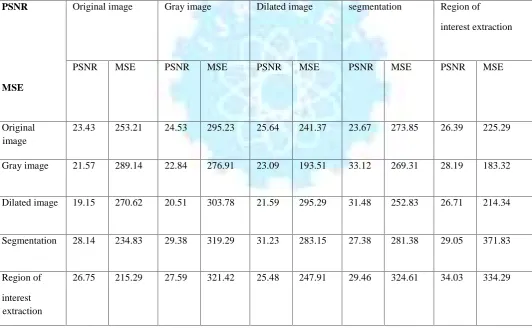
PSNR and MSE for original colour image PSNR
MSE
Original image Gray image Dilated image segmentation Region of
interest extraction
PSNR MSE PSNR MSE PSNR MSE PSNR MSE PSNR MSE
Original image
23.43 253.21 24.53 295.23 25.64 241.37 23.67 273.85 26.39 225.29
Gray image 21.57 289.14 22.84 276.91 23.09 193.51 33.12 269.31 28.19 183.32
Dilated image 19.15 270.62 20.51 303.78 21.59 295.29 31.48 252.83 26.71 214.34
Segmentation 28.14 234.83 29.38 319.29 31.23 283.15 27.38 281.38 29.05 371.83
Region of
interest extraction
[image:9.595.11.544.349.677.2]26.75 215.29 27.59 321.42 25.48 247.91 29.46 324.61 34.03 334.29
www. ijraset.com
Volume 2 Issue IX, September 2014
ISSN: 2321-9653
International Journal for Research in Applied Science & Engineering
Technology(IJRASET)
PSNR and MSE for Steerable image PSNR
MSE
Steerable image Dilated image segmentation Region of
interest extraction
PSNR MSE PSNR MSE PSNR MSE PSNR MSE
Steerable image 29.05 225.29 18.25 274.29 26.75 303.78 22.84 276.91
Dilated image 29.46 269.31 26.72 193.51 28.14 214.34 27.59 247.91
Segmentation 31.23 283.84 26.94 295.23 23.67 334.29 27.59 324.61
Region of
interest extraction
[image:10.595.11.545.91.420.2]27.59 232.49 32.63 295.29 23.09 371.83 23.09 321.42
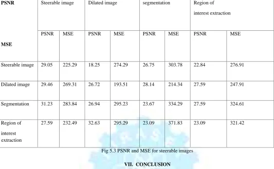
Fig 5.3 PSNR and MSE for steerable images
VII. CONCLUSION
This project deals with the analysis of spatial domain and frequency techniques for license plate detection. We found the performance factors such as PSNR (Peak Signal to Noise Ratio), MSE (Mean Squared Error) for the different types of automobile images with normal colour format. Steerable filter are applied to an image with high possibility for edge detection. Theoretically the images obtained by using steerable filter have a high success ratio for edge detection than that of spatial domain techniques which is evident from the result obtained by us. We also analysed the performance factor when the input image is blurred and tilted. Steerable wavelets provided promising results for blurred and tilted images. With this type of high PSNR and MSE of the Steerable images have high success ratio than normal colour image in every type image such as for a tilted image or a highly blurred image.
REFERENCES
[1] HalinaKwasnicka and BartoszWawrzyniak, “License platelocalization andRecognition in camera pictures”, AI-METH 2002, November 13-15, 2002. [2] ManishaShirvoikar ,”Effective method of license plate localisationand segmentation of vehicles”, May 2013.
[3 P.Sandhya Rani “License plate character segmentation based ondistribution density”IJESAT, Sep-Oct 2012
[4] Khalid W. MagladA “Automobile License Plate Detection and Recognition System” Journal of Computer Science, 2012. [5] PratishthaGupta ,“Number Plate Extraction using Template Matching Technique“, February 2014
[6] SheetalMithunKawade ,“A Real Time Vehicle’s License Plate Recognition System International Journal of Science and Engineering”,2013 .
[7] ManishaRathore ,Tracking number plate from vehicle using matlab,“International Journal in Foundations of Computer Science & Technology” ,May 2014.
[8] I-Chen Tsai,”Recognition of Vehicle License Plates from a Video Sequence”International Journal of Computer Science,17 February 2009
[9] Jun Wei et al ,“Morphology-based license plate detection in image of Differently illuminated and oriented Car” , Journal of electronic imaging, October 15, 2002
[10] William T. Freeman, Edward H. Adelson, “The Design and use of steerable filters”, 1991.