1532
©IJRASET (UGC Approved Journal): All Rights are ReservedCBS - An Efficient & Effective Sensor Node
Deployment Model for Wireless Sensor Network
Er. Vaishyampayan Jain1, Er. Tarun Kumar2
1, 2
Computer Science & Engineering Department, Geeta Institute of Management & Technology, Kanipla, Kurukshetra, Haryana, India
Abstract: Wireless Sensor Network (WSN) is a system consisting of large number of Sensor Nodes (SNs) geographically distributed in the region to be monitored. Sensor is an important part in wireless sensor network. Success of wireless sensor depends upon type, position and situation of sensor nodes. Placement of sensor nodes in deployment area is the major factor that determines the life, coverage area and connectivity of wireless sensor nodes. Most of the events cannot be sensed from distant locations as sensor nodes has limited sensing range. Through literature review, different sensor nodes deployment schemes proposed by the other researchers has been analyzed. Default policy used for the deployment of sensor nodes in the huge area is random deployment. In this paper, authors have suggested a competent and effective sensor deployment model named Cannon Based Scatter. It scatters the sensor nodes using an aerial vehicle over the target region using cannon based scatter design. Proposed design has been tested using Matlab simulator. By minimizing the number of scans required to deploy the sensor nodes, design has shown its effectiveness and efficiency in terms of time, distance and area coverage.
Keywords: Wireless sensor network, Node deployment techniques, Maximum coverage, Network life, Energy, Cannon Based
Scheme.
I. INTRODUCTION
A sensor is a key part of any automatic system. It is an electrochemical unit designed to sense some specific changes happening within its range. There are two types of sensors: (i) Natural (ii) Artificial. Natural sensors exist within the living beings, where signals are generated due to electrochemical changes and communicated via ions through the nerve fibers. Whereas, in artificial sensors (man-made) the signals are generated due to electrochemical or electromechanical changes, but the communication takes place by the flow of electrons through wires. Key characteristics of sensor are bandwidth, resolution, noise, dynamic range, accuracy, sensitivity and transfer function. Sensor unit, processor, memory, battery, energy harvesting module and positioning system are the key components of sensor node [1, 2].
WSN is a system consisting of large collection of Sensor Nodes (SNs) geographically distributed with in the region to be monitored. Key domain of application of wireless sensor node include disaster handling, military surveillance, monitoring of habitat, tracking target, monitoring health of structures, agriculture, intrusion detection and medical monitoring applications. Placement of sensor nodes in deployment area is the major factor that determines the life, coverage area and connectivity of wireless sensor network. Most of the events cannot be sensed from distant locations as sensor node has limited sensing range. This requires sensor nodes to be placed at a distance which is probable location of occurrence of event [3, 4].
The workability of a WSN is measured in terms of three basic parameters: (i) Coverage (ii) Connectivity (iii) life. All of these parameters directly depends on the manner of the placement of SNs within a target region. The process of deployment of SNs within a target region is termed as deployment. The SNs can be deployed manually on pre-computed location if the target region reachable and small-sized. The deployment becomes a tedious task when the target region is uneven, unreachable, vast or hostile [5].
Initially SNs are deployed by dropping from flying machine (helicopter, airplane, etc.) over the deployment area. For this purpose, low cost parachutes are preferably used to ensure safe landing of SNs. Base Station (BS) is mostly placed outside the target area and is considered to have sufficient resources in terms of energy and bandwidth to directly transmit instructions to any SN in the target area. Every SN is considered to have limited communication range (rc) and rs. SN can be mounted on a mobile device to change its physical position in order to adapt the changes required in the network. Deployment can be homogeneous (consisting of SNs with same configuration and capability) or heterogeneous (consisting of SNs with different configurations and capabilities).
1533
©IJRASET (UGC Approved Journal): All Rights are Reservedthe results generated through the simulation. It also contains the analysis of obtained results. Conclusion and future scope are given in section V.
II. LITERATUREREVIEW
[image:3.612.87.525.176.390.2]Classification of techniques of sensor node deployment, are based on the placement strategies, deployment domain, usage, algorithms used and medium of deployment and are summarized in Figure 1.
Fig. 1 Classification of sensor node deployment techniques
Comparative analysis of different node deployment schemes for wireless sensor network found in literature on the relevant parameters is summarized in the table given below:
TABLEI:COMPARATIVE ANALYSIS OF DEPLOYMENT SCHEMES. Scheme Sensor Type Deployment Type Connectivity Type BOS [3] Mobile and static Barrier -
PFM [6] Mobile Full area - VFM [7] Mobile Full area -
CPVF [8] Mobile Full area Multi-path FLOOR [8] Mobile Full area Single-path ORRD [9] Mobile and static Full area Multi-path UAD [10] Static Full area -
CLD [11] Mobile Full area Multi-path CPIM[12] Mobile Point of Interest Single-Path DDS [13] Mobile Full area Multi-path SEEDS[14] Mobile Full area Multi-path
[image:3.612.146.469.452.621.2]1534
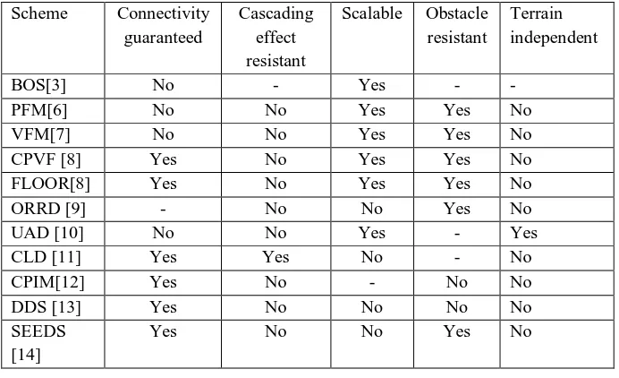
©IJRASET (UGC Approved Journal): All Rights are Reserved [image:4.612.134.480.143.354.2]communication link with sink. Because of the impact on WSNs lifetime Most of the schemes have ignored cascading effect in their discussions but CLD is the only scheme to provide the solution to cascading effect, but the solution is restricted to small area deployments and is not scalable.
TABLE II: Comparative analysis of deployment schemes. Scheme Connectivity
guaranteed
Cascading effect resistant
Scalable Obstacle resistant
Terrain independent
BOS[3] No - Yes - -
PFM[6] No No Yes Yes No
VFM[7] No No Yes Yes No
CPVF [8] Yes No Yes Yes No FLOOR[8] Yes No Yes Yes No
ORRD [9] - No No Yes No
UAD [10] No No Yes - Yes CLD [11] Yes Yes No - No
CPIM[12] Yes No - No No
DDS [13] Yes No No No No SEEDS
[14]
Yes No No Yes No
III.PROPOSEDMODEL
Due to basic characteristics of wireless sensor network, placement of sensor node is a complex task. From the literature review done in the previous section, it was found that sensor nodes were randomly deployed in the region. No specific mechanism was followed for the deployment of sensor nodes. Authors have proposed a model to randomly scatter the sensor nodes from the sky. Main focus in this work was to minimize the value of the following two parameters:
Number of scan required to check the region Time required to deploy the sensor nodes.
Basic terminology and assumptions used for the implementation of the proposed model are as follows:
A. Terminology
1) Dropping rate: Speed with which aerial vehicle move and sensor nodes will be dropped over target region. 2) Aerial Vehicle: It will be used to throw the sensor node over target region.
3) Traceable path: Path to be traced by aerial vehicle over target region for spreading of sensor nodes.
4) Ideal deployment: Target region has been divided in hexagonal shape blocks so that maximum coverage should be achieved through least number of sensor nodes.
B. Assumptions
1) To ensure protection, safe lending and uniform shape of sensor nodes, sensor nodes are embedded inside sphere shape container with a total weight M of .325 kg.
2) Air density ρ has been assumed as constant. Its value is assumed as 1.3 Kg/m3.
3) Number of cannon assumed are 7. So probability of selection of any cannon is 1/7. 4) Length of cannons assumed are {.5, 1.25, 2, 2.75, 3, 3.75, 4}.
C. Construction
1535
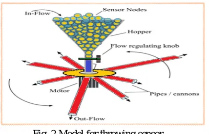
©IJRASET (UGC Approved Journal): All Rights are ReservedFig. 2 Model for throwing sensor
It consists of multiple cannons of different length. A connecting chamber is there to join the one end of all cannons. This is further connected with hopper. This gathering of cannon are connected through a motor to move the cannons. Hopper is filled with sensor nodes and sensor nodes are thrown through rotating cannon in the target area. Different cannon will throw the sensor nodes with different speed. Throwing speed will depend upon the cannon’s length, rotational speed of the motor. Selection of any particular cannon is probabilistic in nature. For small target region, aerial vehicle can stay at a point and throw the sensor nodes through the arrangement shown in figure 2. But if target region is big, then aerial vehicle throws the sensor nodes at different points through the arrangement shown in figure 2.
Length of different cannon are denoted by set Cl = {Cl1, Cl2, Cl3..., Cln}. Now performance of proposed model will be analysed under two different cases
1) Without considering the air resistance 2) By considering the air resistance
D. Without considering the air resistance
If we don’t consider the resistance created by air, then procedure to find the position of sensor node will be as follows: 1) Vinit = speed with which cannon Cli is firing the sensor node = w*Cli (1) 2) w= the rotation speed of motor
3) Cli = the length of i-th cannon
4) Time t for which any sensor will remain in air = (2H/g)1/2 (2) 5) H = represents the height from which sensor was dropped
6) g = the gravitational acceleration (g = 9.8)After releasing sensor will follow the trajectory path which will return coverage of some horizontal distance Dh(li)Dh(li) = w*Cli (2H/g)1/2 (3)
E. By considering the air resistance
When we consider the resistance of air while calculating the exact position of sensor node, then its procedure will be as follows: 1) Fd = Aerial drag force
2) v= speed of the dropped sensor node 3) A = Reference area =3.142*r2
where r is the radius of spherical unit containing sensor node r = [(¾)*(1/3.142) *M]1/3 and M is the mass of spherical unit. 4) ϼ= Air density (1.3 Kg/m3)
5) Cd = Sphere’s drag coefficient (0.476).
6) Fd=1/2v2 (4)Maximum velocity vt achieved by dropped sensor node is given by following formula: 7) vt=(2Mg/ Cd ϼ A)1/2
8) Time required by sensor node to reach at ground is given by following formula:
9) t=(2H/a)1/2Where H represents the height from which sensor was dropped and a represent the gravitational acceleration. Algorithm HD_WAR (H, M, A, vinit)
1536
©IJRASET (UGC Approved Journal): All Rights are Reserved/*This algorithm will calculate the horizontal distance travelled by sensor node while considering the air resistance. Height H from which sensor node of weight M with reference area A was fired with speed vinit has been passed as a parameter to this algorithm*/
t=(2H/a)1/2 x=0; hdist =0; u=vinit = w*Cli Fd=1/2v2ϼ A Cd ah = Fh/M; While (x ≤ t)
{
x++;
v=u+(g-ah)*1; hdist = hdist +v*1; u=v;
}
Return horizontal distance hdist.
IV.RESULTS&ANALYSIS
Proposed CBS model has been tested using Matlab simulator. Its performance has been analyzed on the scale of coverage, distance traveled and time required to cover a region. Also performance has been compared with the uniform airdrop deployment scheme given in [10]. Results are as follows:
[image:6.612.48.556.376.698.2]1537
©IJRASET (UGC Approved Journal): All Rights are ReservedFig. 5 Comparison of region coverage for uniform airdrop scheme [10] and proposed CBS model
Fig. 6 Comparison of distance travelled for uniform airdrop scheme [10] and proposed CBS model
From the analysis of figure 3, 4 and 5, it has been found that proposed CBS model is covering the region in a better manner relative to uniform airdrop scheme [10]
From the analysis of figure 6, it can be concluded that proposed CBS model is travelling very less relative to uniform airdrop scheme [10] while covering region more efficiently. This indicates that proposed CBS model will also take less time for region coverage. Not only time, this also results in less covering cost.
V. CONCLUSIONS
Ordinary approach to sprinkle sensor node in a huge & unfriendly place is random deployment. In this paper, authors have suggested a model named Cannon Based Scatter for deployment of sensor nodes which has been found effective and efficient. Authors have tested the proposed model using code developed in Matlab simulator. Further results have also been analyzed using Matlab tool. It has been found that cannon based scatter is showing better performance on the scale of time, coverage and number of scan required. As a future scope, author has planned to improve the model by using the information of already deployed sensor nodes while dropping the next sensor node at run time.
REFERENCES
[1] B. Black, P. DiPiazza, B. Ferguson, D. Voltmer and F. Berry, “Introduction to wireless systems”, Prentice Hall Press; 2008 May 18.
[2] C. Zhu, C. Zheng, L. Shu and G. Han, “A survey on coverage and connectivity issues in wireless sensor networks”, Journal of Network and Computer Applications. 2012 Mar 31;35(2):619-32.
[3] Z. Sun, P. Wang, M.C. Vuran , M. A. Al-Rodhaan, A. M. Al-Dhelaan and I. F. Akyildiz. “BorderSense: Border patrol through advanced wireless sensor networks”, Ad Hoc Networks. 2011 May 31;9(3):468-77.
[4] V. C. Gungor and G. P. Hancke, “Industrial wireless sensor networks: Challenges, design principles, and technical approaches”, IEEE Transactions on industrial electronics. 2009 Oct;56(10):4258-65.
[5] G. Werner-Allen, K. Lorincz, M. Ruiz, O. Marcillo, J. Johnson, J. Lees and M. Welsh, “Deploying a wireless sensor network on an active volcano”, IEEE internet computing. 2006 Mar;10(2):18-25.
[6] A. Howard, M. J. Mataric and G. S. Sukhatme, “Mobile sensor network deployment using potential fields: A distributed, scalable solution to the area coverage problem”, Distributed autonomous robotic systems. 2002 Jun 25;5:299-308.
[7] Y. Zou and K. Chakrabarty, “Sensor deployment and target localization based on virtual forces. InINFOCOM 2003. Twenty-Second Annual Joint Conference of the IEEE Computer and Communications. IEEE Societies 2003 Mar 30 (Vol. 2, pp. 1293-1303). IEEE.
[8] N. Heo and P. K. Varshney, “A distributed self spreading algorithm for mobile wireless sensor networks”, InWireless Communications and Networking, 2003. WCNC 2003. 2003 IEEE 2003 Mar 20 (Vol. 3, pp. 1597-1602). IEEE.
[9] C.Y. Chang, C.T. Chang, Y.C. Chen and H. R.Chang, “Obstacle-resistant deployment algorithms for wireless sensor networks”, IEEE Transactions on Vehicular Technology. 2009 Jul;58(6):2925-41.
[10] Y. Taniguchi, T. Kitani and K. Leibnitz, “A uniform airdrop deployment method for large-scale wireless sensor networks,”. International Journal of Sensor Networks. 2011 Jan 1;9(3-4):182-91.
[11] Y.S. Yen, S. Hong, R. S. Chang and H. C. Chao, “Controlled deployments for wireless sensor networks”, IET communications. 2009 May 1;3(5):820-9. [12] M. Erdelj, T. Razafindralambo and D. Simplot-Ryl, “Covering points of interest with mobile sensors”, IEEE Transactions on Parallel and Distributed Systems.
2013 Jan;24(1):32-43.
[13] Du, Wenliang, Jing Deng, Yunghsiang S. Han, Shigang Chen, and Pramod K. Varshney. "A key management scheme for wireless sensor networks using deployment knowledge." In INFOCOM 2004. Twenty-third AnnualJoint conference of the IEEE computer and communications societies, vol. 1. IEEE, 2004. [14] Van Dam, T., & Langendoen, K. (2003, November). An adaptive energy-efficient MAC protocol for wireless sensor networks. In Proceedings of the 1st


![Fig. 5 Comparison of region coverage for uniform airdrop scheme [10] and proposed CBS model](https://thumb-us.123doks.com/thumbv2/123dok_us/8306535.856309/7.612.55.557.88.243/comparison-region-coverage-uniform-airdrop-scheme-proposed-model.webp)
