Comparative Performance Analysis of Filtered xLMS and Feedback ANC Adaptive Algorithms to Control the Attenuation of Acoustic Noise

Comparative Performance Analysis of Filtered-xLMS and

Feedback ANC Adaptive Algorithms to Control the

Attenuation of Acoustic Noise

Tushar Kanti Roy

Department of Electronics and Telecommunication Engineering, Rajshahi University of Engineering & Technology, Rajshahi-6204 *Corresponding Author: roy_kanti@yahoo.com

Copyright © 2013 Horizon Research Publishing All rights reserved.

Abstract

performance analysis of two adaptive algorithms to control the attenuation of acoustic noise. Active noise control (ANC) is one of the most popular applications for adaptive filters. The basic idea behind the active control of acoustic noise is to inject a secondary sound (anti-noise) into an environment so as to cancel the primary sound using destructive interference. So, ANC is a method of reducing the unwanted noise by actively generating an anti-noise, cancelling out the noise. To achieve this objective, throughout this paper, I describe two well-known filtered-x least Mean Square (filtered-x LMS) and feedback active noise control algorithms which provide a new structure for improving acoustic noise reduction. Finally, from the simulation results, it is obvious that the proposed adaptive algorithms can effectively control the acoustic narrowband noise from the corrupted speech signal.

Keywords

Noise Control (ANC), Filtered-Xlms Adaptive Filter, Feedback ANC, MSE

1. Introduction

In our increasingly mobile society, individuals are lying on your front to doing just about everything on the move. Listening music is certainly not an exception. However, when anyone listens to music away from the home, anyone necessarily has less control over noise exposure. Airplane, bus, and car engines are the most common noise distractions as one travels. Lawn mower engines, others’ speech and music are also frequently encountered. Hence, it is necessary to find ways to reduce such unwanted noise. Active noise cancellation (ANC) is a method for reducing undesired noise from the desired signal. This is (ANC) achieved by introducing a canceling “anti-noise” wave through secondary sources. This secondary source is interconnected

through an electronic system using a specific signal processing algorithm for the particular cancellation scheme. Throughout this paper, we build a noise-cancelling headphone by means of active noise control. There are a number of great applications for active noise cancellation devices. Noise cancellation almost requires the sound to be cancelled at a source, such as from a loudspeaker. One application is such that people working near aircraft or in noisy factories can now wear these electronic noise cancellation headsets to protect their hearing. The noise signal usually comes from any device, such as a rotating machine, so that it is possible to measure the noise near me this source. Therefore, the goal of the active noise control system is to produce an "anti-noise" that attenuates the unwanted noise in a desired quiet region using an adaptive filter. Due to recent advances in wireless technology, new applications of the ANC have emerged, e.g., incorporating ANC in cell phones, Bluetooth headphones, and MP3 players, to mitigate the environmental acoustic noise in order to improve the speech and music quality [5]. A conventional adaptive algorithm such as the LMS algorithm is likely to be unstable in this application due to the phase shift (the delay) introduced by the forward path [1, 2]. The well-known filtered-XLMS-algorithm is, however, an adaptive filter algorithm which is suitable for active control applications [3]. It is developed from the LMS algorithm, where a model of the dynamic system between the filter output and the estimate, i.e., the forward path is introduced between the input signal and the algorithm for the adaptation of the coefficient vector [3, 4]. Implementation of active noise control system using NLMS adaptive algorithm is proposed in [5]. In order to control the wideband noise from the speech signal a higher order x-LMS filter is proposed in [6]. Therefore, the main contribution of this paper is to control the acoustic narrowband noise from the speech signal via ANC using Filtered-xLMS and feedback ANC adaptive algorithms.

describes the NLMS algorithm and adaptive Feedback ANC is described in subsection A. The simulation results of the proposed algorithms are presented in Section III. Finally the paper concludes in Section IV.

2. Adaptive Filter Structure

This section describes the framework of an adaptive filter algorithm. As the characteristics of the acoustic noise source and the environment are time varying, the frequency content, amplitude, phase, and sound velocity of the undesired noise are non-stationary. Therefore, in order to cope with these variations the ANC system must be adaptive. The most common form of adaptive filter is the transversal filter using the least mean-square (LMS) algorithm. Fig.1 shows a framework of adaptive filter. Basically, there is an adjustable filter with input X and output Y. Our objective is to minimize the difference between‘d’ and ‘Y’, where‘d’ is the desired signal. Once the difference is computed, the adaptive algorithm will adjust the filter coefficients with that difference. There are many adaptive algorithms available in the literature, the most popular ones being LMS (least mean-square) and RLS (Recursive least squares) algorithms. In the interest of computational time, we used the LMS.

Figure 1. Adaptive filter framework

Figure 2. Adaptive Filter Using Least Mean Square

NLMS Algorithm

Adaptive filter is still an active research area that plays an important role in an ever increasing number of applications, such as noise cancellation, channel estimation, channel

equalization and acoustic echo-cancellation etc. There are many adaptive algorithms available but among these algorithms the least mean square (LMS) approach is widely used for adaptive filter routines. This algorithm does not require squaring, averaging, or differentiating. The LMS algorithm provides an alternative method for determining the optimum filter coefficients. The block diagram of an adaptive filter is shown in Fig. 2.

The least mean square (LMS) algorithm, which is given by

)

(

)

(

2

)

(

)

1

(

n

B

n

e

n

x

n

k

b

+

=

+

β

−

where,

)

(

)

(

)

(

n

d

n

y

n

e

=

−

The output of the adaptive filter is given by

)

(

)

(

0

B

x

n

k

n

y

k k

−

=

∑

= (2)

Adaptive Feedback ANC Basics

Adaptive Noise Cancellation (ANC) is a widely applicable set of noise attenuating techniques. Unlike simple filtering, ANC techniques attenuate noise through the addition of an “anti-noise” signal with 180-degree phase difference, thereby dampening the energy of the noise waves. Active feedback via an embedded microphone facilitates targeted noise cancellation without any requisite a priori knowledge about the signal transmitted or the noise present. The single-channel adaptive feedback ANC system works by processing the acoustical noise that we would like to reduce (the “target” noise), and then it produces an anti-noise which is sent into the air, thus attenuating the target noise at a particular point in space (in our case this is the space adjacent to the error microphone). Therefore, the goal of the ANC system is to minimize the signal received by the error microphone. In Fig. 3, the residual waveform is what is picked up by the microphone.

Figure 3. The Single-Channel Feedback ANC System; a generalized concept.

Figure 4. Physical description of active noise control

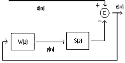
The feedback ANC system produces an anti-noise by predicting the incoming target noise. This is not different from an adaptive system identification scheme; to achieve this; the system uses the Least-Mean Squares (LMS) algorithm to update an adaptive filter coefficients which are the heart of ANC signal processing. As shown in Fig. 5, the target noise d[n] is not available because it is intended to be canceled by the anti-noise. Our goal is that we want to create an anti-noise y[n] which predicts the inaccessible d[n]. Therefore, one task of the feedback ANC algorithm is to estimate d[n] and use it as the reference signal x[n] for the adaptive filter W(z). (Notice that y[n] is in the electrical domain, and in order to cancel d[n] it must go through the speaker and the air: this is modeled by secondary path filter S(z).)

Figure 5. Simplified block diagram of single-channel feedback ANC system.

In Z-domain, the target signal can be expressed as

),

(

)

(

)

(

)

(

z

E

z

S

z

Y

z

D

=

+

Where, E(z) is the error signal picked up by the microphone, and Y(z) is the anti-noise generated by the adaptive W(z) filter. If the secondary path S(z) is measurable (expressed as S^_{(z)), then we can estimate the target noise d[n] (let us call}

this the synthesized x[n]).

)

(

)

(

)

(

)

(

)

(

z

D

z

E

z

S

z

Y

z

X

_≡

₌

₊

Therefore, the algorithm achieves its first task, which is to regenerate the reference signal x[n] ≡ d^_[n].

For completeness, in time domain (2) is expressed as

∑

= ∧ ∧

−

+

=

≡

0

]

[

]

[

]

[

]

[

m m

m

n

y

s

n

e

n

d

n

x

Where s^m, m = 0, 1, … , M-1 are the secondary-path IIR

filter coefficients. The next task is to create the anti-noise y[n] from x[n] such that the error signal e[n] is minimized. We employ the filtered-x LMS algorithm to do this.

Figure 6. Adaptive feedback ANC system using the F-xLMS algorithm

The anti-noise is generated as

∑

=

−

=

0

]

[

]

[

]

[

l

w

n

x

n

l

n

y

where wl, l = 0, 1, … , L-1 are the coefficients of W(z). These

coefficients are updated according to the filtered-x LMS algorithm, which is expressed as

1

,...,

1

,

0

],

[

]

[

]

[

]

1

[

_n

₊

₌

_w

_n

₊

_x

_n

₋

_l

_e

_n

_l

₌

_L

₋

w

µ

where µ is the step size, and

∑

=

−

=

0 ^

'

_[

_]

_[

_]

m m

m

n

x

s

n

x

This is the filtered x[n].

3. Simulation Results

This section presents the simulation results of the proposed algorithms. Noise cancellation makes use of the notion of destructive interference. When two sinusoidal waves superimpose, the resulting waveform depends on the frequency amplitude and relative phase of the two waves. If the original wave and the inverse of the original wave encounter at a junction at the same time, total cancellation occurs. The challenges are to identify the original signal and generate the inverse without delay in all directions where noises interaction and superimpose. For this active noise control, we use a sampling frequency of 8 KHz and noise frequency ranging from 100 to 800 Hz.

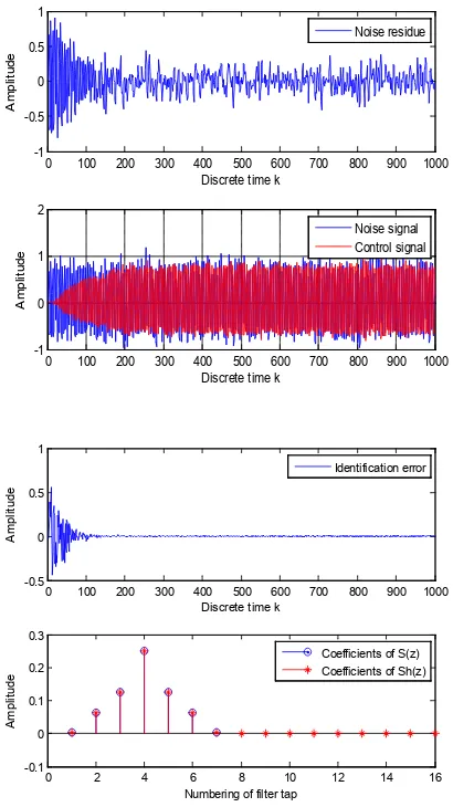
the Feedback control algorithm almost received the exact control signal to cancel the noise i.e., the error signal is zero.

Figure 7. Simulated output using a Feedback ANC algorithm

The secondary signal propagation path is the path the anti-noise takes from the output loudspeaker to the error microphone within the quiet zone. The above Fig.8 shows the impulse response using the true secondary path.

Figure 8. Impulse response using the true secondary path

The first task in active noise control is to estimate the impulse response of the secondary propagation path. This step is usually performed prior to noise control using a synthetic random signal played through the output loudspeaker while the unwanted noise is not present. The Fig.9 shows the coefficients of the true, error and estimated path. The impulse response estimation can be generated for secondary path.

Figure 9. Impulse Response estimation of Secondary Path

Typically, the length of the secondary path filter estimate is not as long as the actual secondary path and need not be in adequate control in most cases. The normalized LMS algorithm is used due to its simplicity and robustness. The Fig.10 represents the output and error signals of NLMS algorithm show that the algorithm converges after about 10000 iterations.

Figure 10. Use of the adaptive filter for secondary identification

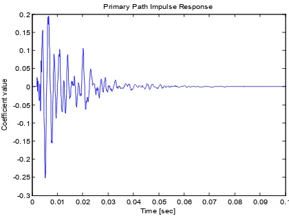
The Impulse response of the primary propagation path of the noise to be cancelled can also be characterized by a linear filter. The Fig.11 shows the Impulse response of the primary path.

0 100 200 300 400 500 600 700 800 900 1000 -1

-0.5 0 0.5 1

A

m

pl

itude

Discrete time k

Noise residue

0 100 200 300 400 500 600 700 800 900 1000 -1

0 1 2

A

m

pl

itude

Discrete time k

Noise signal Control signal

0 100 200 300 400 500 600 700 800 900 1000 -0.5

0 0.5 1

A

m

pl

itude

Discrete time k

Identification error

0 2 4 6 8 10 12 14 16

-0.1 0 0.1 0.2 0.3

A

m

pl

itude

Numbering of filter tap

Coefficients of S(z) Coefficients of Sh(z)

0 0.01 0.02 0.03 0.04 0.05 0.06 0.07 0.08 0.09 0.1 -0.4

-0.3 -0.2 -0.1 0 0.1 0.2 0.3

Time [sec]

C

oef

fic

ient

v

al

ue

True Secondary Path Impulse Response

0 0.01 0.02 0.03 0.04 0.05 0.06 0.07 0.08 0.09 0.1 -0.4

-0.3 -0.2 -0.1 0 0.1 0.2 0.3

Time [sec]

C

oef

fic

ient

v

al

ue

Secondary Path Impulse Response Estimation

True Estimated Error

0 0.5 1 1.5 2 2.5 3

x 104 -4

-3 -2 -1 0 1 2 3 4 5

Number of iterations

S

ignal

v

al

ue

Secondary Identification Using the NLMS Adaptive Filter

Figure 11. Impulse Response of Primary path

Typical active noise control applications involve the sounds of rotating machinery due to their annoying characteristics. Here, we synthetically generated a noise that might come from a loudspeaker.

Figure 12. Power spectral density of the noise to be cancelled

Figure 13. Use of filtered-x LMS adaptive Controller for active noise control

Listening to its sound at the error microphone before cancellation, it has the characteristic industrial “whine” of such loudspeaker. The spectrum of the sound is also plotted that shown in Fig. 12. The most popular adaptive algorithm for active noise control is the filtered-xLMS algorithm. This algorithm uses the secondary path estimate to calculate an output signal whose contribution at the error sensor destructively interferes with the undesired noise. The reference signal is a noisy version of the undesired sound measured near its source. The resulting algorithm converges after about 5 seconds of adaptation. Listening to the error signal, the annoying “whine” is reduced considerably which is shown in Fig. 13.

Figure 14. Power spectral density of the original and attenuated noise

Comparing the spectrum of the residual error signal with that of the original noise signal, we can see that most of the periodic components have been attenuated considerably. However, the steady-state cancellation performance may not be uniform across all frequencies. Such is often the case for real-world systems applied to active noise control tasks.

Figure 15. MSE decay versus time sample for proposed methods.

0 0.01 0.02 0.03 0.04 0.05 0.06 0.07 0.08 0.09 0.1 -0.3

-0.25 -0.2 -0.15 -0.1 -0.05 0 0.05 0.1 0.15 0.2

Time [sec]

Coef

fic

ient

v

al

ue

Primary Path Impulse Response

0 0.2 0.4 0.6 0.8 1 1.2 1.4 1.6 1.8 2

-70 -60 -50 -40 -30 -20 -10 0

Frequency (kHz)

P

ow

er

/fr

equenc

y (

dB

/H

z)

Power Spectral Density of the Noise to be Cancelled

0 1 2 3 4 5 6

x 104 -4

-3 -2 -1 0 1 2 3 4

Number of iterations

S

ignal

v

al

ue

Active Noise Control Using the Filtered-X LMS Adaptive Controller

Original Noise Anti-Noise Residual Noise

0 200 400 600 800 1000 1200 1400 1600 1800 2000 -70

-60 -50 -40 -30 -20 -10 0

Frequency (Hz)

P

ow

er

/fr

equenc

y (

dB

/H

z)

Power Spectral Density of the Original and Attenuated Noise

Original Attenuated

0 200 400 600 800 1000 1200 1400 1600 1800 2000 10-4

10-3 10-2 10-1

100

Time Index

S

qu

a

re

d

E

rr

or

V

al

u

e

4. Conclusion

In this paper, ANC mechanism is utilized using filtered x-LMS and Feedback ANC adaptive algorithms to control the acoustic narrowband noise from the corrupted speech signal. Blocking low frequency has the priority since most real life noises are under 1 KHz, for example engine noise or noise from aircraft. This mainly led me to focus my project on low frequency noise cancellation. More specifically, the ANC headset can deal with noise frequency ranging from 100 Hz to 800 Hz. Throughout this paper, I have implemented and compared two variations of adaptive algorithms, namely Filtered-xLMS and Feedback ANC to control the acoustic noise. From the simulation results, it is obvious that the proposed adaptive algorithms can effectively control the acoustic narrowband noise from the corrupted speech signal.

REFERENCES

[1] S.J. Elliott and P.A. Nelson, “Active noise control,” IEEE signal processing magazine, pages 12–35, October 1993. [2] D.R Morgan “An analysis of multiple correlation

cancellation loops with a filter in the auxiliary path,” IEEE Transactions on Acoustics, Speech and Signal Processing, ASSP-28(4):454–467, August 1980.

[3] P.A. Nelson and S.J. Elliott, “Active Control of Sound,” Academic Press, Inc, 1992.

[4] B. Widrow and S.D. Stearns, “Adaptive Signal Processing,” Prentice-Hall, 1985.

[5] G.P.Kadam and Saba Fatima, “Implementation of active noise control system using multi-rate digital signal processing technique,” World Journal of Science and Technology 2012, 2(5):15-20.