Asset Market Dynamics in Equilibrium Models
with Heterogeneous Agents: Analytical Results
P. M. Beaumont
1,∗,
A. J. Culham
2,
A. N. Kercheval
31Department of Economics, Florida State University, Tallahassee, Florida, 32306, United States
2Constellation Energy, Baltimore, Maryland, United States
3Department of Mathematics, Florida State University, Tallahassee, Florida, 32306, United States
∗Corresponding Author: [email protected]
Copyright c⃝2013 Horizon Research Publishing All rights reserved.
Abstract
We examine market dynamics in a discrete-time, Lucas-style asset-pricing model with heteroge-neous, utility-optimizing agents. Finitely many agents trade a single asset paying a stochastic dividend. All agents know the probability distribution of the dividend but not the private information such as wealth and asset holdings of other agents. The market clearing price is determined endogenously in each period such that sup-ply always equals demand.Our aim is to determine whether and how the pricing function evolves toward equilibrium. In the special case where all agents have logarithmic utility, but possibly different holdings and discount factors, we completely describe the market dynamics, including the evolution of the pricing and demand functions, and asset holdings of the agents. The market converges to a stable equilibrium state where only the most patient agents remain, and the equilibrium pricing function is the same as the one arising in the simple homogeneous setting.
Keywords
Market Dynamics, Market Disequilib-rium, Correct Expectations Equilibrium1
Introduction
In a general equilibrium asset pricing model, the exis-tence of a rational expectations equilibrium (REE) im-plies that each trader solves a utility-optimization prob-lem that incorporates all current information about the market. In particular, traders implicitly must: (i) have full knowledge of the problem including knowing the preferences and holdings of all the other agents, (ii) be able to deduce their optimal behavior no matter how complex, and (iii) share common expectations includ-ing that all the other agents are themselves rational and know all these things. In a sense, these agents must be “super-rational”: they are “experienced masters” in a stable world where the past is a good indicator of the fu-ture, and full rationality of all agents is common
knowl-edge [1, ch. 1].
Access to full information has the advantage of mak-ing the REE, in many cases, unique and computation-ally feasible [2]. However, real traders seldom know this much, because real markets are always changing unpre-dictably. Since super-rational agents cannot evolve, we also cannot use the REE concept to study market states away from equilibrium, or the dynamics of convergence toward equilibrium. Important prior work on REE-style equilibrium models, including [3, 4, 5], has naturally fo-cused solely on the equilibrium states themselves and do not illuminate the nearby disequilibrium states and their evolution, which are typical initial states for boundedly-rational agents.
The agent-based computational economic (ACE) modeling literature, where agents follow formal, often myopic, rules, which can evolve by natural selection takes a more general, econophysical view of market dy-namics [6, 7, 8]. This literature examines the result-ing emergent properties of the market, includresult-ing the dy-namics of prices and holdings as the market evolves and agents with poor rules die and those with good rules prosper. These systems are typically studied by simula-tion. An excellent and recent review of this literature is provided in [9].
In this paper we study a discrete-time, general equi-librium Lucas tree economy with one asset and N >1 infinitely lived agents who act to optimize an infinite-horizon utility. The asset (stock) is in fixed supply and pays a random dividend in each period. The asset price is determined endogenously in each period such that to-tal (price-dependent) demand is equal to toto-tal supply. The dividend is assumed to follow a Markov process whose distribution is known to the agents, but we need make no further assumptions about it – it’s distribution may be discrete or continuous.
Agents determine how much to consume and how much to invest in the stock each period by optimizing a time-separable constant relative risk aversion (CRRA) utility function. As in the standard Lucas model, at any time, agent i, 1 ≤ i ≤ N, holds a certain num-ber of shares of stocksi ≥0, which can vary over time
if the agent trades. (Short positions are not allowed.) Agents also have discount factors βi and risk-aversion
parameter γi. All of which are allowed to vary across
the population of agents.
Our agents are “boundedly rational” in the specific sense that they do not know the holdings or parameters of the other agents. Therefore they cannot incorporate that information into the solution of their personal op-timization problems. As we will see, this allows us to model the economy both at and away from equilibrium. To compute their optimal asset demand and con-sumption functions each agent must solve an expecta-tion involving future market-clearing prices. Tomor-row’s market clearing price P′ depends on tomorrow’s unknown dividendD′ (the only source of randomness in our model). While agents know the probability distri-bution ofD′, they do not know how the market clearing priceP(D′) depends onD′ since this depends in part on the behavior of other agents.
Therefore, solving for the demand equations requires agents, individually, to hypothesize “best guess” market-clearing pricing functions pi(D′). This allows them to
compute optimal demands, conditional onpi(·), and to
trade if indicated. The market will actually clear to-day at a pricePm(D), such that supply equals demand.
(Here we make explicit the dependence ofPm(·) on the
dividendD, but in general, in disequilibrium, this func-tion also depends on all the agents’ holdings, parame-ters, and pricing functionspi [2].)
Using the terminology from [1], we will say that the market is at a “correct expectations equilibrium” (CEE), if all agents are using the same pricing function Pm(·)
to solve for optimal demand, and this pricing function is correct in the sense that the actual resulting market clearing price isPm(D) in every period. This framework
has the advantage that agent behavior is well-defined whether or not the market is at equilibrium.
We may now ask whether CEE exist in our framework and, if so, whether they are unique and how we can characterize market dynamics. Specifically, how do the asset holdings and market clearing pricing function Pm
evolve over time,both at and awayfrom equilibrium? In general, we do not expect to find closed formulas describing the dynamics of such markets and so would investigate these questions via numerical simulation, as is common in the ACE literature. However, we can give rigorous and complete answers to these questions in the special (but reasonable) case where all agents have log utility (γi= 1).
In summary, we will find that there is a unique CEE pricing function given by
P∗(D) = β
1−βD, (1)
whereβ is the discount factor of the most patient agent. CEE stock holdings are zero for agents with discount fac-tor less thanβ, and can be distributed arbitrarily among
agents with discount factor equal to β. This result is consistent with the long-known principle (e.g. [3]) for REE equilibria that the most patient agent eventually holds all the wealth. Our work confirms this principle in the CEE boundedly rational context typical of ACE and furthermore we provide a formal proof of conver-gence to the familiar pricing function well-known in the homogeneous case.
Finally, we formally prove that asset holdings and market pricing functions evolve according to explicit for-mulas given below (equations (11), (12)). The market dynamics do not depend on the individual pricing func-tionspi, on the learning mechanism used, if any, or on
the probability distribution of dividends. Each CEE is a fixed point of the dynamics. From any disequilibrium initial condition, markets will converge deterministically and exponentially fast to a CEE given by equations (1) and (15). Therefore we are able to use methods of deter-ministic dynamics to analyze the evolution in this paper, rather than the statistical methods used in many ACE models with stochastic inputs.
Since [3] there has been a renewed interest in the role of heterogeneous discount rates in determining market dynamics. In his 2011 Presidential address to the Amer-ican Finance Association, Cochrane [10] emphasizes the importance of discount rates in discussing many of the “puzzles” in asset pricing. The role of discount rate het-erogeneity in explaining wealth inequality is discussed by [11], [12, 13] focus specifically on heterogeneity of time preferences and asset prices, and [14] considers the effects of heterogeneous patience on the terms structure of interest rates. An interesting example of how hetero-geneous rates of time preference can help describe per-sonal behaviors such as the decision to smoke is given in [15]. Our work contributes to this literature by adding a formal mathematical analysis of the dynamical behav-ior of asset markets in a general equilibrium model with heterogeneous agents.
2
Model framework
Consider the standard Lucas asset pricing model [16, 17] withN possibly heterogeneous agents and a sin-gle risky asset with period t market clearing spot price denoted Pt. The number of shares of the asset is
nor-malized to beN and the asset pays a random dividend
Dtper share, described by some Markov process and so
determined solely by the observed state of the world at the beginning of each period t. All agents are assumed to know the distribution of dividend payments across states, which can be arbitrary, discrete or continuous, stationary or not.
There is no production in this economy so in time periodtagentiwill choose optimal consumptionci,t ≥0
and investment in the asset si,t+1 ≥ 0 based upon the agent’s preferences and period budget constraint
ci,t+Ptsi,t+1≤wi,t= (Pt+Dt)si,t, for allt, (2)
wherewi,t is the agent’s periodtwealth.
The order of events is as follows. Agentibegins period
t knowing her asset holdings si,t. Next, today’s stock
agent does not yet know her current wealth because the market pricePthas yet to be determined through market
clearing. Each agent must first compute her optimal demand as a function of price, si(P), representing the
optimal number of shares demanded at any given price
P. These demand functions then collectively determine the unique pricePtthat clears the market according to
N
∑
i=1
si(Pt) =N. (3)
The actual mechanism of market clearing is not impor-tant; we can imagine that there is some market maker who collects the demand functions from each agent and publicly declares the market price satisfying (3). (This price will be unique if, for example, demands are all monotone inP.) This declared market price is the only source of information about the other agents.
Each agent is assumed to be an expected utility max-imizer with constant relative risk aversion preferences and risk aversionγi>0. The one-period utility of
con-sumption is
ui(c) =
c1−γi−1
1−γi
, γi̸= 1,
or
ui(c) = logc, γi= 1,
and consumption and investment polices must be found that optimize the time-separable expected utility
max {ci,τ, si,τ+1}∞τ=t
Et
∞
∑
τ=t
βiτ−tui(ci,τ) (4)
subject to the budget constraint (2). The agents’ dis-count factors,βi∈(0,1), may differ and the expectation
in (4) is over the distribution of dividends and is con-ditional upon the information available to the agent at the beginning of periodt.
Denote by st ∈ RN the vector of all agents’ time-t
asset holdings. We explicitly include the time subscript to emphasize that these holdings may change over time. We describe two different equilibrium concepts which we label REE and CEE.
Definition 1 A rational expectations equilibrium
(REE) for this economy consists of an aggregate pricing function P∗(Dt,st) for the risky asset and a set of
agent consumption demand functions ci,t = ci(Dt,st)
and asset demand functions si,t+1 = si(Dt,st) such
that, for all future times t, the asset market clears at
Pt = P∗(Dt,st), the budget constraint is satisfied for
each agent, and the demand functions solve the agents’ optimization problems (incorporating full knowledge of the market).
Our boundedly rational agents, however, do not know
st, and must optimize based upon more limited
knowl-edge. Therefore we use instead the notion of a CEE:
Definition 2 A correct expectations equilibrium
(CEE) for this economy consists of an aggregate pric-ing function P∗(Dt) for the risky asset and a set of
agent consumption demand functions ci,t =ci(Dt, si,t)
and asset demand functions si,t+1 = si(Dt, si,t) such
that, for all future times t, the asset market clears at Pt = P∗(Dt), the budget constraint is satisfied
for each agent, and the demand functions solve the agents’ optimization problems (incorporating available knowledge).
To clarify the difference between “available knowl-edge” and “full knowlknowl-edge”, we need to look at the op-timization problem more carefully.
Solving the Bellman equation from the usual recur-sive dynamic programing approach leads to the following standard Euler equation as viewed from time t, which must be satisfied by the optimal consumption demand functionci,t+1:
Pt=Et
[
βi
(
ci,t+1
ci,t
)−γi
(Pt+1+Dt+1)
]
. (5)
Using the budget constraint (2) to eliminate c, and using the notation s′i,t = si,t+1 = si(Dt, si,t), and
s′′i,t = si(Dt+1, si,t+1) = si(Dt+1, si(Dt, si,t)), we may
rewrite (5) as
Pt=βEt
[(
si,t(Pt+Dt)−s′i,tPt
s′i,t(Pt+1+Dt+1)−s′′i,tPt+1
)γi
(Pt+1+Dt+1)
]
. (6)
Each agent, at equilibrium, must solve for the asset de-mand functionsi(D, s) that satisfies this optimality
con-dition.
Now our boundedly rational agents will have a prob-lem computing the conditional expectation in the Eu-ler equation because they need to know the equilibrium pricing function P∗ in order to know the probability distribution of tomorrow’s prices which depends on the holdings and preferences of the other agents. Worse, it depends on knowing that the other agents also know the equilibrium pricing function, which will not be true in disequilibrium.
For illustration, consider a simple case where agents are super-rational and the REE is computable. Suppose all agents are identical with log utility (βi =β, γi = 1,
si,t = 1, for alliandt) and all agents are aware of this.
Knowing they are identical, agents can deduce that there will never be any trading and so the budget constraint will thus imply that ci,t =Dt and si,t+1 =si,t = 1 for
each agent. The Euler equation (5) simplifies to
Pt=Et
[
βi
(
Dt
Dt+1
)
(Pt+1+Dt+1)
]
(7)
which is now easy to solve. The REE aggregate pricing function satisfying this equation is
P∗(Dt) =
β
1−βDt.
and holdings s= (s1, . . . , sN) remain fixed over time.
equilibrium so the REE pricing function, and hence the market clearing price, is known by all agents as soon as the dividend is announced so there is no need to compute demand functions for a range of prices. This is a signif-icant simplification of the problem, but its operational validity is questionable: only if the agents know that all other traders are identical to themselves can they justify settingci,t =Dtin their Euler equation [18].
In our boundedly rational world, agents do not know holdings or preferences of the other agents, nor what pricing functions the other agents are using. Therefore they cannot know whether the market is at equilibrium. They can only know whether their own pricing function is correctly predicting market clearing prices.
Our way forward is to allow agents to use private es-timates pi(Dt+1) of the period t+ 1 aggregate pricing
function in their Euler equations (5). We assume that these functions depend uponD alone. Although agents are aware that there are unobserved variables st and
functions {pj}j̸=i influencing market prices away from
equilibrium, we can imagine they implicitly operate un-der the hypothesis that the market will converge to a CEE, so that the dependence on these variables will van-ish with time. Thus, it is pragmatic for the agents to usepi(Dt+1) in the Euler equation.
At a CEE, the demand functions si depend only on
current holdings si,t and the current dividend Dt,
be-cause the asset pricePtis implicitly determined by Dt.
Away from equilibrium this is no longer the case. In order for a market clearing price to be determined ac-cording to equation (3), each agent’s demand function must include price Pt as an explicit independent
vari-able. In other words,agents must determine how much
to demand at any potential price. These demand
equa-tions will then determine the current period’s market clearing price, and, in turn, each agent’s actual realized investment.
This framework now provides agents with enough in-formation to derive optimal consumption and asset de-mand functions ci,t = ci(Dt, si,t, P|pi) and si,t+1 =
si(si,t, Dt, P|pi), where we indicate explicitly the
de-pendence on the choice of pricing function pi, which
is allowed to change over time, e.g. via some learning mechanism.
Now we can make precise the spaces and dynamics we are studying.
• Let D be the set of possible dividends and P the set of possible asset prices; in this case both can be taken to be the setR+of nonnegative real numbers.
• Pwill denote the set of all possible pricing functions
p : D → P. This can be thought of as a space of random processes depending on the underlying dividend processDt.
• S ⊂ RN is the set of all possible holdings vectors
s= (s1, . . . , sN)
• A = PN is the set of possible vectors of agents’
individual pricing functions (p1, . . . , pN).
The market clearing functionM :S × A → P, given the agents’ holdings and pricing functions, returns the
resulting market clearing pricing function implied via (3) by the resulting agents’ optimal demand functions.
Themarket dynamical state spaceis
X ={(s, p,a)∈ S × P × A:M(s,a) =p}.
An element of X specifies asset holdings s, individual pricing functions a, and the resulting market pricing function p. (Note we suppress the space D, since the underlying dividend process is exogenous; effectively we are studying the dynamics of random processes measur-able with respect to the filtration generated by{Dt}.)
Themarket dynamical systemis the mappingf :X →
X corresponding to updating the state variables by one time step. The holdings vector s will change due to trading and the vectora of agent pricing functions will change due to the particular learning mechanism chosen, if any. The passage of time is tracked by the trajectory of an f-orbit {fn(x) : n = 0,1,2,3, . . .} of an initial
state x∈ X, where fn denotes the n-fold composition
off with itself.
In this framework, a CEE corresponds to a state (s, p∗,a) where a = (p∗, p∗, . . . , p∗) and f(s, p∗,a) = (s′, p∗,a) for somes′. If there is no trading, then (s, p,a) will be a fixed point off.1
We will now focus on a special case where it is possible to derive tractable analytical results.
3
The log utility case
Suppose all N >1 agents have CRRA utility with a common risk aversion,γi=γ >0 for all i, but possibly
differing discount factorsβi and initial holdings si,0. We assume the aggregate supply of stock isN shares, and that agents have limited information in the sense that they may not make any assumptions about the pref-erences or holdings of the other agents when solving for their optimal consumption in each time period. Agents are presumed to have private estimatespi(·) of the
pric-ing function, but we impose no assumptions yet on what these are or how they evolve.
Using the budget constraint to substitute for c, the
ith agent’s Euler equation (5) is given by the following equation, where for convenience we use the notationD=
DtandD′=Dt+1:
P
(si,t(P+D)−P si(D, si,t, P))γi
=βiEt
[(
pi(D′) +D′
)
/
(
si(D, si,t, P)
(
pi(D′) +D′
)
−pi(D′)si(D′, si(D, si,t, P), pi(D′))
)γi
]
. (8)
Here, P represents any current market price,si,t is the
time-t number of shares of stock of agent i, pi is the
ith agent’s current pricing function, and si(D, s, P) is
the ith agent’s optimal demand function, which is the unknown here. The agent’s optimization problem is to find a functionsi satisfying (8) for all possible values of
1If there is perpetual trading at equilibrium, none of these
points will be fixed, but we could view a CEE as the smallest
P; the actual market price will be determined after all agents have done this.
Notice that the unknown demand functionsiappears
in (8) in a highly nonlinear way. Nonetheless, agents must solve this equation for si in order to be able to
participate in the implicit price-calling auction used to arrive at the market clearing price. (Though this poses a computational problem in simulations, we assume our agents can solve this mathematical problem at no cost.) In the log-utility case (γi= 1), it is easy to verify that
(8) has the simple explicit solution
si(D, s, P) =βi
(
1 + (D/P))s. (9) Unlike the general caseγi̸= 1, this solution has the
spe-cial property that it does not depend upon the agent’s pricing functionpi. This is a very important feature of
log utility and is what makes this special case analyti-cally tractable.
Because the pricing functionspido not influence agent
behavior, the specific learning mechanism used by the agent to update her pricing function guess is rendered irrelevant, and the dynamical system f projects down to a mapping
g:Y →Y
on thereduced dynamical state space
Y ={(s, p)∈ S × P: (s, p,a)∈X for somea∈ A},
consisting of just asset holdings and market clearing price functions.
The market clearing price, which we now denotePm=
Pm(Dt), is determined from the market clearing
condi-tion
N
∑
i=1
si(si,t, Dt, Pm) =N. (10)
Substituting the demand function (9) forsi and solving
for the market clearing price, gives
Pm=
∑N
1 βjsj
N−∑N1 βjsj
D. (11)
Substituting (11) into the demand function (9) gives the agent’s next period holdings at market clearing prices as
si,t+1=si(si,t, D, Pm) =βi
(
N
∑N
1 βjsj,t
)
si,t. (12)
The evolution of holdings has now become a deter-ministic dynamical system h : S → S given by h = (h1, . . . , hN) where
hi(s1,t, . . . , sN,t) =βi
(
N
∑N
1 βjsj,t
)
si,t. (13)
At any time, the market pricing function Pm is
deter-mined by the asset holdings according to (11), so the market dynamical system is completely described byh. We now need only determine the behavior ofh-orbits on
S in order to completely understand the time evolution of our market.
The following theorem establishes that this dynamical system converges and reports the limiting asset holdings and pricing function.
Theorem 1 Consider a pure exchange economy of N
infinitely-lived agents and N shares of a single risky as-set paying stochastic dividendDat the beginning of each period. Each agent maximizes her discounted, expected life-time utility subject to the period budget constraint
ci+P s′i ≤(P +D)si. All agents have log utility and
have discount factors βi and initial asset holdings s◦i,
where ∑Ni=1s◦i =N. Agents know the probability distri-bution of dividends but not the asset holdings, discount factors, or utility functions of other agents.
For convenience, order the agents by decreasing dis-count factor and letkbe the number of agents who share the maximum discount factor β, so that
1> β=β1=· · ·=βk > βk+1≥ · · · ≥βN >0.
Then the dynamic behavior of holdings and market clearing prices is given by the deterministic equations (11) and (12). This system converges exponentially fast to
P∗(D) = β
1−βD (14)
and
s∗i = N s ◦
i
s◦1+· · ·+s◦k, i≤k, (15a)
= 0, i > k. (15b) The theorem states that the asset holdings of all agents with less than the maximum subjective discount factor converge to zero at an exponential rate. The as-set holdings of the remaining most patient agents, with the highest discount factor, converge to a limit propor-tional to the initial holdings of this subset of agents. The patience of these agents is eventually rewarded by accumulating all of the wealth in the economy while the impatient agents are driven out of the market as their wealth is asymptotically driven to zero. Furthermore, the economy eventually collapses to a set of agents with differing holdings but a common discount factor. The market clearing price globally converges to the pricing function obtained in the classical and more restricted case of homogeneous, super-rational agents.
In the special case where agents (unknowingly) have identical discount factors but possibly different initial holdings, there is never any trading and the market clears immediately in the first time step at the famil-iar rational expectations equilibrium price
Pm=
β
1−βD. (16)
3.1
Proof of Theorem 1Proof: It is easy to verify algebraically that the de-mand function (9) solves the Euler equation (8), and therefore (11) and (12) describe the market clearing price and new stock holdings in each time step.
Also, it is easy to see that the market clearing price
Pm is given by the P∗ in (14) if the stock holdings are
such that the only non-zero holdings are for agents with
βi = β. Therefore it remains to prove that holdings
It is convenient to rewrite the dynamical system (13) in terms of the relative holdingsxi=si/N:
x′i =∑βNixi 1 βjxj
. (17)
Here xj ∈ [0,1] for all j and
∑
jxj = 1, so the state
(x1, . . . , xN) lies on the (N−1)-dimensional unit simplex
∆N ={(x1, . . . , xN)≥0 :
∑
i
xi= 1} (18)
in the positive orthant ofRN. Since ∑jx′j= 1, we can describe the dynamics as an iteration of the mapping
T : ∆N → ∆N where the ith coordinate of T(x) is
defined to bex′i given by (17).
If Γ⊂∆N denotes thek-dimensional simplicial face
Γ ={(x1, . . . , xk,0, . . . ,0) : k
∑
j=1
xj = 1}, (19)
then it is easy to see that every point of Γ is fixed byT. From (17), if xj ̸= 0 andβi =βj, then T(xi)/T(xj) =
xi/xj. HenceT always preserves the relative sizes of the
coordinates x1, . . . , xk. Therefore the limiting holdings
must be given by (15) if we can show that every forward
T-orbit{Tn(x)}converges to Γ.
Define πΓ : ∆N → Γ to be the projection fixing the firstkcoordinates and setting the remainingN−k co-ordinates to zero. Let ∆N+={x∈∆N :π
Γ(x)̸= 0}.
Lemma 2 Define F : ∆N → R by F(x) = ∑iβixi,
where β =β1 and the βi are ordered as in Theorem 1.
Then for anyx∈∆N+, F(Tn(x)) increases monotoni-cally with limit β asn→ ∞.
Proof: Let Υ denote the (N −k)-dimensional sub-simplicial face
Υ ={(0, . . . ,0, xk+1, . . . , xN) : N
∑
j=k+1
xj= 1}, (20)
andπΥ : ∆N →Υ the projection fixing the last N−k coordinates and setting the firstkto zero.
F(x) is is simply a weighted average of the β’s, weighted by thex’s.
Using the definition ofT, we have, for anyx,
F(T(x)) =
∑
iβ
2
ixi
F(x) (21) and so F(x)F(T(x)) = ∑iβ2
ixi. Also, F2(x) =
(∑iβixi)2.
NowF(T(x))≥F(x) follows from Jensen’s inequality
ϕ(∑
i
βixi)≤
∑
i
ϕ(βi)xi (22)
for the convex function ϕ(x) = x2. The inequality is strict if bothπΓ(x) andπΥ(x) are nonzero.
Fix x ∈ ∆N+. If π
Υ(x) = 0 then x ∈ Γ, T(x) =
x, and F(x) =β, so there is nothing further to prove. Hence supposeπΥ(x) is nonzero. This meansπΓ(T(x)) andπΥ(T(x)) are also nonzero, soF(Tn(x)) is a strictly
monotone sequence bounded by β. It must therefore converge to it’s supremum, call itβ∗.
Supposeβ∗< β. By compactness of ∆N, the sequence
{Tn(x)} has a convergent subsequence y
k =Tnk(x)→
x∗ ∈ ∆N, and by continuity of F, F(x∗) = β∗. By the definition of T, (Tn(x))i is monotone increasing for
i = 1, . . . , k. Therefore x∗ ∈∆N+. Since F(x∗) < β,
πΥ(x∗)̸= 0, and so
F(T(x∗))> F(x∗) =β∗. (23) However, we also haveF(T(yk))≤β∗, and sinceyk →
x∗this contradicts the continuity ofF andT. Therefore we must haveβ∗ =β. This completes the proof of the lemma.
From the lemma above, the limit ofF(Tn(x)) isβ for
all x∈ ∆N+. SinceF is continuous and F−1(β) = Γ, every forward T-orbit starting in ∆N+ must converge to Γ. From equation (12), we see that if holdings are close to zero for agentsj =k+ 1, . . . , N, then we have, approximately,
s′j= βj
β1
sj, (24)
which gives us, asymptotically, an exponential rate of convergence to zero all j > k. This completes the proof of Theorem 1.
3.2
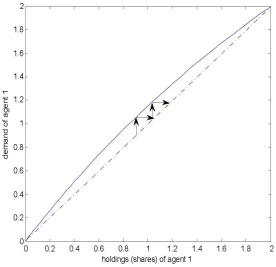
An Illustration with Two AgentsFor the special case of two agents with different dis-count factorsβ1> β2 it is possible to describe the mar-ket dynamics with a simple diagram. The asset demand functions are
si(s1,t, s2,t) =βi
2si,t
β1s1,t+β2s2,t
, i= 1,2. (25) Using the market clearing constraints1,t+s2,t= 2 gives
s1(s1,t) =
β1s1,t
β2+ (β1−β2)(s1,t/2)
(26a)
and
s2(s2,t) =
β2s2,t
β1+ (β2−β1)(s2,t/2)
. (26b)
Figure 1. For a market with two agents having different discount factors β1 = 0.95 andβ2 = 0.7, we plot the demand function
of agent 1 (solid), and the diagonal (dashed). The demand function of agent 2 is symmetrically below the diagonal because of the market-clearing requirements1+s2= 2. Iteration of agent 1’s demand function, describing the passage of time, is illustrated with the
arrows. Holdings for agent 1 converge to 2. Symmetrically, holdings for agent 2 converge simultaneously to zero.
Iteration of the upper function for agent 1, the most patient agent with the higher discount factor, is illus-trated with the arrows showing that asset holdings will converge to s = 2. Similarly, the asset holdings of the less patient agent 2 will decrease monotonically to zero along the lower function. This behavior is common to any choice of discount factors as long asβ1> β2. When
β1=β2both graphs are along the diagonal and the as-set holdings of both agents remain fixed and there is no trading.
4
Conclusions
Theorem 1 and the surrounding discussion provide the details of the answers summarized in the Introduction. Since, in our log-utility case, the decisions of the agents turn out to be uninfluenced by the chosen pricing func-tions a ∈ A, the full dynamical system f : X → X
conveniently reduces to a mappingg:Y →Y on the re-duced state space. This allows us to completely specify the market dynamics both at and away from equilib-rium.
Our model is fully consistent with a rational expecta-tions general equilibrium framework and does not rely upon agents who ignore market fundamentals or behave irrationally such as in [20, 19]. At each period in our model markets clear according to (10) which sets the aggregate demand for assets equal to the aggregate sup-ply. The market price is then determined endogenously according to (11) which depends upon the individual as-set demand equations of each agent.
We are able to completely specify the asset market dynamics of this system as the economy moves toward
equilibrium. We show that the most patient agents will asymptotically accumulate all wealth with a convergence rate that depends upon the ratio of the discount factor of the less patient agent to the most patient agent. In an environment without idiosyncratic wealth shocks, this convergence will be monotonic. Although our conclu-sions are consistent with the existing literature we have provided a rigorous proof of these results.
It’s natural to ask about what happens when agents are allowed to have other risk aversion parameters γi >
0. In general, optimal demands will then depend on the individual pricing functionsaas well as the wealth and asset holdings distributions [2]. Therefore, the mapping
f :X →X will not be fully specified until the pricing function updating (learning) mechanism is specified.
Simulation studies are reported in [21] for this gen-eral case where the learning mechanism is a simple least squares updating of the pricing function based on the observed history of market prices. In all cases studied, market prices are observed to converge to a no trad-ing equilibrium which, in our language, is a fixed point (s, P∗,a) off :X →X, wherea= (P∗, . . . , P∗). These simulation studies are numerically challenging because each agent’s optimal demand must be solved numeri-cally in every time step.
The log utility case makes for an interesting compar-ison between our two equilibrium concepts, CEE and REE. Assuming that agents know all the pricing func-tions, holdings, and preferences of the other agents will not change their behavior in each time step. Equations (11) and (12) describe the market price Pm(D,s) and
Pm(D) evolves over time and reaches the equilibrium
P∗(D) only in the limit.
Acknowledgements
This work is partially supported by the FSU Council on Research and Creativity, IDS grant #014895. The authors are grateful for the helpful suggestions of the anonymous referee.
REFERENCES
[1] Magill, M. and Quinzii, M. Theory of Incomplete Markets, volume 1. MIT Press, 1996.
[2] Miao, J. Competitive equilibria of economies with a continuum of consumers and aggregate shocks. Journal of Economic Theory, Vol. 128, No. 1, 274 – 298, 2006.
[3] Becker, R. A. On the Long-Run Steady State in a Simple Dynamical Model of Equilibrium with Hetero-geneous Households. Quarterly Journal of Economics, Vol. 95, No. 2, 375–382, 1980.
[4] Hern´andez D., A. and Santos, M. Comptetiive Equi-libria for Infinite-Horizon Economies with Incomplete Markets. Journal of Economic Theory, Vol. 71, 102– 130, 1996.
[5] Magill, M. and Quinzii, M. Incomplete Markets Over an Infinite Horizon: Long-Lived Securities and Spec-ulative Bubbles. Journal of Mathematical Economics, Vol. 26, 133–170, 1996.
[6] Palmer, R. G., Arthur, W. B., Holland, J. H., LeBaron, B., and Tayler, P. Artificial Economic Life: A Simple Model of a Stockmarket. Physica D: Nonlinear Phe-nomena, Vol. 75, No. 1–3, 264–274, 1994.
[7] Arthur, W. B., Holland, J. H., LeBaron, B., Palmer, R., Tyler, P. Asset Pricing Under Endogenous Expecta-tions in an Artificial Stock Market. In: Arthur, W. B., Durlauf, S. N., Lane, D. A. (Eds.), The Economy An an Evolving Complex System II. Addison-Wesley, pp. 15–44, 1997.
[8] Chiarella, C., Dieci, R., Gardini, L. Asset Price and Wealth Dynamics in a Financial Market with Heterogeneous Agents. Journal of Economic Dynamics and Control, Vol. 30, 1755–1786, 1998.
[9] Chiarella, C., Dieci, R. and He, X-Z. Heterogeneity, Market Mechanisms, and Asset Price Dynamics. In: Thorsten Hens IV and Klaus Reiner Schenk-Hoppe,
editors, Handbook of Financial Markets: Dynamics and Evolution, Ch. 5, 277–344, North-Holland Amsterdam, 2009.
[10] Cochrane, J. H.Presidential address: Discount rates. The Journal of Finance, Vol. 66, No. 4, 1047–1108, 2011.
[11] Hendricks, L. How important is discount rate hetero-geneity for wealth inequality?. Journal of Economic Dynamics and Control, Vol. 31, No. 9, 3042–3068, 2009.
[12] Gollier, C., Zeckhauser, R. Aggregation of heteroge-neous time preferences. Journal of Political Economy, Vol. 113, No. 4, 878–896, 2005.
[13] Lengwiler, Y., Malamud, S., Trubowitz, E. Asset pricing in heterogeneous economies. ETH Zurich Department of Mathematics Working Paper, 2005.
[14] Lengwiler, Y. Heterogeneous patience and the term structure of real interest rates. The American Economic Review, Vol. 95, No. 3, 890–896, 2005.
[15] Scharff, R. L., Viscusi, W. K. Heterogeneous rates of time preference and the decision to smoke. Economic Inquiry, Vol. 49, No. 4, 959–972, 2011.
[16] Lucas, Jr, R. E., Asset prices in an exchange economy. Econometrica, Vol. 46, No. 6, 1429–1445, 1978.
[17] Lyungqvist, L., Sargent, T. J., Recursive Macroe-conomic Theory, 2nd Edition. The MIT Press, Cambridge, MA, 2004.
[18] Frydman, R. Individual rationality and decentraliza-tion. In: Roman Frydman and E. S. Phelps, editors, Individual Forecasting and Aggregate Outcomes: Rational Expectations Examined, Ch. 5, pp. 97–122, Cambridge University Press, UK, 1984.
[19] Guidolin, M., Timmermann, A. Properties of equilib-rium asset prices under alternative learning schemes. Journal of Economic Dynamics and Control, Vol. 31, 161–217, 2007.
[20] Jouini, E., Napp, C. Heterogeneous beliefs and asset pricing in discrete time: An analysis of pessimism and doubt. Journal of Economic Dynamics and Control, Vol. 30, 1233–1260, 2006.