Modified Fault Tolerant Double Tree Network 2

Modified Fault Tolerant Double Tree Network-2

Gagandeep Kaur

lecturer,Department Of Computer Applications Lovely Professional University

Phagwara

Sandeep Sharma

Associate professor, Department of computer science & engineering

Guru Nanak Dev University Amritsar.

ABSTRACT

Interconnection networks are constructed to provide inter-process communication. These Networks are compared on the basis of Fault tolerance, Reliability, Path length and cost effectiveness. An irregular class of Fault Tolerant Multistage Interconnection Network (MIN) called Modified Four Double Tree Network-2 (MFDOT-2) is proposed.MFDOT-2 is constructed on the basis of FDOT-2 [1]. The Reliability, Path length and cost effectiveness of some popular irregular class of Multistage Interconnection Networks along with proposed MFDOT-2 is also analyzed.

Keywords

Four Double Tree Network (FDOT-2); Modified Four Double Tree Network-2 (MFDOT-2); Four Tree Network (FT)

1.

INTRODUCTION

Network MFDOT-2 is being proposed which is better than FDOT-2 network with respect to Reliability, Path length and cost effectiveness and is as good as other similar networks.

2.

MFDOT-2

MFDOT-2 is modified network of FDOT-2 [1] network as shown in Figure 1. In the network all 2 X 2 switches are used, stages 0 & 1 has similar no of switches i.e. N/2. At stage 1 the no of switches are N/2+2. The no of MUX and DEMUX used are 5*n+4. There are redundant paths available in the network that enhances its fault tolerant property. There are two independent fully connected networks of 8 x 8 size; they are then connected with the addition of 4 switches. It gives better path length, bandwidth on lower cost and comparable Reliability with the corresponding MDOT-2 network.

3.

ANALYSIS

3.1

Reliability Analysis

Both Upper Bond and Lower Bond reliability analysis [2-3] are being shown for the fault tolerant irregular multistage interconnection networks.

3.1.1. Lower Bound Analysis

The SEs of input stage and multiplexers are integral part. The reliability black diagram is shown in figure 2.

RL-MFDOT-2(t)=[1-(1-e–t)] (N/4-1)]. [1-(1-e–t)] (N/4-1)].[1-(1-e–

t

)2](N/2-1) ]

MTTF=∞0∫ RL-MFDOT-2 (t) . d(t)

Figure2. Lower Bound Reliability Block Diagram of

MFDOT-2

N/4-1 Copies (N/4-1)Copies N/2-1 Copies SEm

SEm

SEm

SEm

SEm

SEm SE

SE

3.2 Path Length Analysis

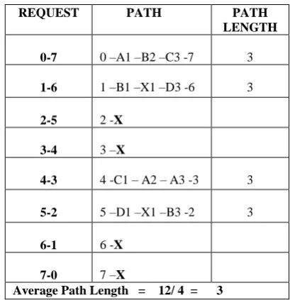
Path length refers to the length of the communication path between the sources to destination. Multiple paths of different path lengths are possible in a network .It can be measured in distance or by the number of intermediate switches. The possible path lengths [4] between a particular pair of source to destination may vary from 2 to maximum number of stages. The various path lengths of some popular networks along with proposed network is calculated to route a data from given source to destination is shown in the following tables

 X is used in case no further path is available and the request has to be dropped.

 In path the character represents the switch and the digit represent the stage in which it exists.

3.2.1

without Fault

BEST CASE

REQUEST PATH PATH

LENGTH

0-0 0 -A1 –A3 -0 2

1-1 1 –B1 –X1 –B3 -0

3

2-2 2 –B1 –A2 –A3 -2

3

3-3 3 –X

4-4 4 –C1 –C3 -4 2

5-5 5 –D1 –X1 –D3 -5

3

6-6 6 –D1 –B2 –C3 -6

3

7-7 7 –X

Average Path Length = 16 / 6 = 2.6 AVERAGE CASE

REQUEST PATH PATH

LENGTH

0-1 0 -A1 –A3-1 2

1-3 1 –B1 –A2 –A3 -3 3

2-5 3 -B1 –X1 –D3 -5 3

3-7 3 –A1 –B2 –C3 -7 3

4-0 4 –X

5-2 5 –D1 –X1 –B3 -2 3

6-4 6 –C1 –C3 -4 2

7-6 7 -D1 –B2 –X

Average Path Length = 16 / 6 = 2.6 WORST CASE

REQUEST PATH PATH

LENGTH

0-7 0 –A1 –B2 –C3 -7 3

1-6 1 –B1 –X1 –D3 -6 3

2-5 2 -X

3-4 3 –X

4-3 4 -C1 – A2 – A3 -3 3

5-2 5 –D1 –X1 –B3 -2 3

6-1 6 -X

7-0 7 –X

Average Path Length = 12/ 4 = 3

Table 1.1 Different cases for without fault specifications

3.2.2 With 1 MUX failure

BEST CASE

REQUEST PATH PATH

LENGTH

0-0 0 –B1 –A2 –A3 -0 3

1-1 1 –X

2-2 2 –A1 –A3 -2 2

3-3 3 –B1 –X1 –B3 -3 3

4-4 4 –C1 –C3 -4 2

5-5 5 –D1 –X1 –D3 -5 3

6-6 6 –D1 –B2 –C3 -6 3

7-7 7 –X

Average Path Length = 16 / 6 = 2.6

AVERAGE CASE

REQUEST PATH PATH

LENGTH

0-1 0 –B1 –A2 –A3 -1 3

1-3 1 –X

2-5 3 -B1 –X1 –D3 -5 3

3-7 3 –A1 –B2 –C3 -7 3

4-0 4 –C1 –X

6-4 6 –C1 –C3 -4 2

7-6 7 -D1 –B2 –X

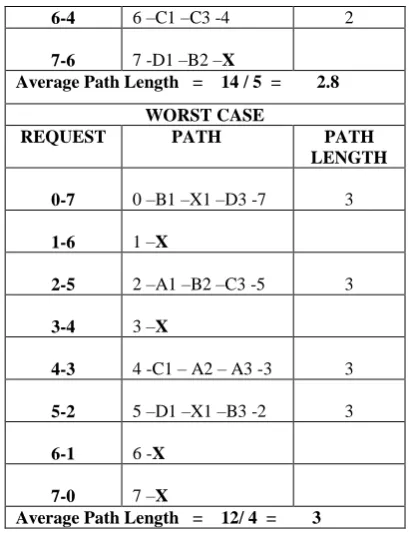
Average Path Length = 14 / 5 = 2.8

WORST CASE

REQUEST PATH PATH

LENGTH

0-7 0 –B1 –X1 –D3 -7 3

1-6 1 –X

2-5 2 –A1 –B2 –C3 -5 3

3-4 3 –X

4-3 4 -C1 – A2 – A3 -3 3

5-2 5 –D1 –X1 –B3 -2 3

6-1 6 -X

7-0 7 –X

Average Path Length = 12/ 4 = 3

Table 1.2 Different cases for with 1MUX failure

specifications

3.2.3

with Failure of 1 Switch at Level 1

BEST CASE

REQUEST PATH PATH

LENGTH

0-0 0 –B1 –A2 –A3 -0 3

1-1 1 –X

2-2 2 –B1 –X1 –B3 -2 3

3-3 3 –X

4-4 4 –C1 –C3 -4 2

5-5 5 –D1 –X1 –D3 -5 3

6-6 6 –D1 –B2 –C3 -6 3

7-7 7 –X

Average Path Length = 16 / 6 = 2.6 AVERAGE CASE

REQUEST PATH PATH

LENGTH

0-1 0 –B1 –A2 –A3 -0 3

1-3 1 –X

2-5 3 -B1 –X1 –D3 -5 3

3-7 3 –X

4-0 4 –D1 –X1 –B3 -0 3

5-2 5 –D1 –X1 –B3 -2 3

6-4 6 –C1 –C3 -4 2

7-6 7 -D1 –B2 –X

Average Path Length = 14 / 5 = 2.8 WORST CASE

REQUEST PATH PATH

LENGTH

0-7 0 –B1 –X1 –D3 -7 3

1-6 1 –X

2-5 2 –X

3-4 3 –X

4-3 4 -C1 – A2 – A3 -3 3

5-2 5 –D1 –X1 –B3 -2 3

6-1 6 -X

7-0 7 –X

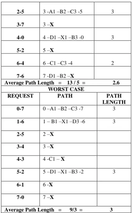
Average Path Length = 9/3 = 3

Table 1.3 Different cases With Failure Of 1 Switch At

Level 1 specifications

3.2.4

with Failure of 1 Switch at Level 2

BEST CASE

REQUEST PATH PATH

LENGTH

0-0 0 –A1 –A3 -0 2

1-1 1 –B1 –X1 –B3 -1 3

2-2 2 –X

3-3 3 –X

4-4 4 –C1 –C3 -4 2

5-5 5 –D1 –X1 –D3 -5 3

6-6 6 –D1 –B2 –C3 -6 3

7-7 7 –X

Average Path Length = 13 / 5 = 6

AVERAGE CASE

REQUEST PATH PATH

LENGTH

0-1 0 –A1 –A3 -1 2

2-5 3 -A1 –B2 –C3 -5 3

3-7 3 –X

4-0 4 –D1 –X1 –B3 -0 3

5-2 5 –X

6-4 6 –C1 –C3 -4 2

7-6 7 -D1 –B2 –X

Average Path Length = 13 / 5 = 2.6 WORST CASE

REQUEST PATH PATH

LENGTH

0-7 0 –A1 –B2 –C3 -7 3

1-6 1 – B1 –X1 –D3 -6 3

2-5 2 –X

3-4 3 –X

4-3 4 -C1 – X

5-2 5 –D1 –X1 –B3 -2 3

6-1 6 -X

7-0 7 –X

Average Path Length = 9/3 = 3

Table 1.4 Different cases with Failure Of 1 Switch At Level

2 specifications

Table 1.5 RESULTS OF ABOVE ANALYSIS

Result With Respect To 8 Requests

R.M Average

Path Length

Without fault

Best Case

6 2.6

Average Case

6 2.6

Worst Case

4 3

With MUX Faulty

Best Case

6 2.6

Average Case

5 2.8

Worst Case

4 3

With 1 Switch Faulty At Level 1

Best Case

5 2.8

Average Case

5 2.8

Worst Case

3 3

With 1 Switch Faulty At Level 2

Best Case

5 2.6

Average Case

5 2.6

Worst Case

3 3

3.3 Cost Effectiveness

A measure of cost effectiveness [4] for reliability can be given by comparing MTTF and the cost of the network. Various Assumptions:

Component Cost (units)

Switch (2 x 2) 4

Switch (4 x4) 16

Mux (m: 1) / Demux (m: 1) m

No of Components Cost(units)

Switches (2 x 2) 26 104

Mux 24 48

Demux 24 48

Total cost 200

Table 1.6

3.4 Bandwidth Analysis

Probability of acceptance (Pa) =0.9634

P req.gen BW

0.1 0.2 0.3 0.4 0.5 0.6 0.7 0.8 0.9 1.0

1.540 3.080 4.620 6.160 7.700 9.240 10.78 12.32 13.86 15.41

3.5 Performance Comparison

MFODT-2 is better in terms of Reliability, Path length and cost effectiveness of FDOT-2 network, and is almost comparable and equivalent in performance to other networks such as FT [4], MFT [5], ZETA [6-7] and IASN [5] networks.

 Path Length

The Maximum Path length ofFDOT-2 network is 5

The Maximum path length of FT network is 5 The Maximum Path length of ZETA network is

5

The Maximum Path length of IASN network is 3

The Maximum Path length of MFDOT-2

network is 3

Clearly MFDOT-2 has better performance than

FDOT-2 network in terms of average path length.

 Bandwidth

Pa B.W

FDOT-2 0.687 10.9

FT 0.687 10.9

ZETA 0.687 10.9

MFDOT-2 0.9 15.41

Table 1.8

Clearly the Bandwidth of MFDOT-2 network is more than FDOT-2 network.

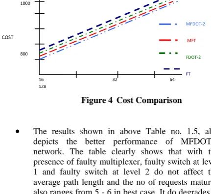
 Cost Effectiveness

The Total Cost of FDOT-2 network is 252 units The Total Cost of FT network is

258 units The Total cost of MFT is

240 units The Total Cost of ZETA network is

256 units The Total Cost of IASN network is

239 units

The total cost of MFDOT-2 is 200 units

MFDOT-2 is less costly than FDOT-2 network. It cannot be

exactly compared with other networks with respect to cost effectiveness as FT, MFT, ZETA and IASN are complete fault tolerant networks. MFDOT-2 network can be easily made fault tolerant but with little more cost than these fully fault tolerant networks.

 The results shown in above Table no. 1.5, also depicts the better performance of MFDOT-2 network. The table clearly shows that with the presence of faulty multiplexer, faulty switch at level 1 and faulty switch at level 2 do not affect the average path length and the no of requests matured also ranges from 5 - 6 in best case. It do degrades in worst case in which requests matured ranges from 3-4.

4. REFERENCES

[1] Bansal P.K., Singh K.Joshi R.C., “Fault Tolerant Double Tree Multistage Interconnection Network” in: Proceedings of int. Conference IEEE INFOCOM, april 1991, pp.462-468

[2] Reibman A.L., (1991), “Failure dependant performance analysis of a fault tolerant MIN” , in: Proceedings of IEEE Transaction on reliability, vol. 40, no. 4, 1991, pp. 461-473.

[3] Somani A.K., vaidya N.H., (1997), “Understanding fault tolerance and reliability”, Computer. vol. 30, no. 4, April 1997

[4] Bansal P.K., Singh K.Joshi R.C., “Routing and Path Algorithm for cost Effective Four Tree Multistage Interconnection Network”, Int. J. of electronics, Vol. 73 No. 1, 1992, pp 107-115.

[5] Harsh Sadawarti, P.K. Bansal,, “Fault Tolerant Irregular Augmented Shuffle Network” proceeding of the 2007 WSEAS Inetrnational Conference on computer enginnering and application, Gold Cost Australia, January 17-19,2007.

[6] Bansal P.K., Singh K.Joshi R.C., “Quad Tree: a cost effective Fault Tolerant `Multistage Interconnection Network” IEEE INFOCOM, April 1991, pp. 860-866, may 4-8, 1992.

[7] Shoman, M.L., “Reliability of computer systems and networks:fault tolerance, analysis, and design. “Johan Wiley &Sons, Inc., New York 2002.

COST

16 32 64 128

N

1000

800

600

400

200

MFDOT-2

MFT

FDOT-2

FT