R E S E A R C H
Open Access
A modified subgradient extragradient
method for solving monotone variational
inequalities
Songnian He
1,2*and Tao Wu
1*Correspondence:
1College of Science, Civil Aviation
University of China, Tianjin, 300300, China
2Tianjin Key Laboratory for
Advanced Signal Processing, Civil Aviation University of China, Tianjin, 300300, China
Abstract
In the setting of Hilbert space, a modified subgradient extragradient method is proposed for solving Lipschitz-continuous and monotone variational inequalities defined on a level set of a convex function. Our iterative process is relaxed and self-adaptive, that is, in each iteration, calculating two metric projections onto some half-spaces containing the domain is involved only and the step size can be selected in some adaptive ways. A weak convergence theorem for our algorithm is proved. We also prove that our method hasO(1n) convergence rate.
MSC: 47J20; 90C25; 90C30; 90C52
Keywords: variational inequalities; subgradient extragradient method; Lipschitz-continuous mapping; level set; half-spaces; convergence rate
1 Introduction
LetH be a real Hilbert space with inner product·,·and norm · . The variational inequality problem (VIP) is aimed to finding a pointx∗∈C, such that
fx∗,x–x∗≥, ∀x∈C, (.)
whereCis a nonempty closed convex subset of H andf :C→H is a given mapping. This problem and its solution set are denoted byVI(C,f) andSOL(C,f), respectively. We also always assume thatSOL(C,f)=∅. The variational inequality problemVI(C,f) has re-ceived much attention due to its applications in a large variety of problems arising in struc-tural analysis, economics, optimization, operations research and engineering sciences; see [–] and the references therein.
It is well known that the problem (.) is equivalent to the fixed point problem for finding a pointx∗∈C, such that []
x∗=PC
x∗–λfx∗, (.)
whereλis an arbitrary positive constant. Many algorithms for the problem (.) are based on the fixed point problem (.). Korpelevich [] proposed an algorithm for solving the
problem (.) in Euclidean spaceRn, known as the extragradient method (EG):
x∈C,
˜
xn=PCxn–λf(xn), (.)
xn+=PCxn–λf(xn˜ ), (.)
whereλis some positive number andPCdenotes the metric projection ofHontoC. She proved that iff isκ-Lipschitz-continuous andλis selected such thatλ∈(, /κ), then the two sequences{xn}and{˜xn}generated by the EG method, converge to the same point z∈SOL(C,f).
In , Nadezhkina and Takahashi [] generalized the above EG method to general Hilbert spaces (including infinite-dimensional spaces) and they also established the weak convergence theorem.
In each iteration of the EG method, in order to get the next iteratexk+, two projections ontoCneed to be calculated. But projections onto a general closed and convex subset are not easily executed and this might greatly affect the efficiency of the EG method. In order to overcome this weakness, Censoret al.developed the subgradient extragradient method in Euclidean space [], in which the second projection in (.) ontoCwas replaced with a projection onto a specific constructible half-space, actually which is one of the subgradient half-spaces. Then, in [, ], Censoret al.studied the subgradient extragradient method for solving theVIPin Hilbert spaces. They also proved the weak convergence theorem under the assumption thatf is a Lipschitzian continuous and monotone mapping.
The main purpose of this paper is to propose an improved subgradient extragradient method for solving the Lipschitz-continuous and monotone variational inequalities de-fined on a level set of a convex function [], that is,C:={x∈H|c(x)≤}andc:H→R is a convex function. In our algorithm, two projectionsPC in (.) and (.) will be re-placed withPCk andPTk, respectively, whereCkandTkare half-spaces, such thatCk⊃C
andTk⊃C.Ckis based on the subdifferential inequality, the idea of which was proposed firstly by Fukushima [], andTkis the same one as Censor’s method [].
It is also worth pointing out that the step size in our algorithm can be selected in some adaptive way, that is, we have no need to know or to estimate any information as regards the Lipschitz constant off, therefore, our algorithm is easily executed.
Our paper is organized as follows. In Section , we list some basic definitions, proper-ties and lemmas. In Section , the improved subgradient extragradient algorithm and its corresponding geometrical intuition are presented. In Section , the weak convergence theorem for our method is proved. Finally, we prove that our algorithm hasO(n) conver-gence rate in the last section.
2 Preliminaries
In this section, we list some basic concepts and lemmas, which are useful for constructing the algorithm and analyzing the convergence. LetH be a real Hilbert space with inner product·,·and norm · and letC be a closed convex subset ofH. We writexk
PC(x), such that
x–PC(x)≤ x–y, ∀y∈C. (.)
The mappingPC:H→Cis called the metric projection ofHontoC. It is well known that PCis characterized by the following inequalities:
x–PC(x),PC(x) –y≥, (.)
x–y≥x–PC(x)+y–PC(x), (.)
for allx∈H,y∈C[, ].
A function c:H→Ris said to be Gâteaux differentiable atx∈H, if there exists an element, denoted byc(x)∈H, such that
lim
t→
c(x+tv) –c(x)
t =
v,c(x), ∀v∈H,
wherec(x) is called the Gâteaux differential ofcatx. We saycis Gâteaux differentiable onH, if for eachx∈H,cis Gâteaux differentiable atx.
A functionc:H→Ris said to be weakly lower semicontinuous (w-lsc) at x∈H, if xkximpliesc(x)≤lim infk→∞c(xk). We saycis weakly lower semicontinuous onH, if for eachx∈H,cis weakly lower semicontinuous atx.
A functionc:H→Ris called convex, if we have the inequality
ctx+ ( –t)y≤tc(x) + ( –t)c(y),
for allt∈[, ] andx,y∈H.
For a convex functionc:H→R,cis said to be subdifferentiable at a pointx∈Hif the set
∂c(x)d∈H|c(y)≥c(x) +d,y–x,∀y∈H (.)
is not empty, where each element in∂c(x) is called a subgradient ofcatx,∂c(x) is subdiffer-ential ofcatxand the inequality in (.) is said to be the subdifferential inequality ofcatx. We saycis subdifferentiable onH, ifcis subdifferentiable at eachx∈H. It is well known that ifcis Gâteaux differentiable atx, thencis subdifferentiable atxand∂c(x) ={c(x)}, namely,∂c(x) is just a set of the simple points [].
A mappingf :H→His said to be Lipschitz-continuous [], if there exists a positive constantκ, such that
f(x) –f(y)≤κx–y, ∀x,y∈H.
f is also said to be aκ-Lipschitzian-continuous mapping. A mappingf :H→His said to be monotone onH, if
Definition .(Normal cone) We denote the normal cone byNC(v) [] ofCatv∈C,
i.e.
NC(v) :=w∈H| w,y–v ≤,∀y∈C. (.)
Definition .(Maximal monotone operator) LetT:H⇒Hbe a point-to-set operator defined onH.Tis called a maximal monotone operator ifTis monotone,i.e.
u–v,x–y ≥, ∀u∈T(x) and∀v∈T(y)
and the graphG(T) ofT,
G(T) :=(x,u)∈H×H|u∈T(x),
is not properly contained in the graph of any other monotone operator.
It is clear that a monotone mappingTis maximal iff for any (x,u)∈H×H, ifu–v,x– y ≥,∀(y,v)∈G(T), then it follows thatu∈T(x).
Define
Tv=
⎧ ⎨ ⎩
f(v) +NC(v) ifv∈C, ∅, ifv∈/C.
ThenT is maximal monotone and ∈Tvif and only ifv∈SOL(C,f) [].
The next property is known as the Opial condition and all Hilbert spaces have this prop-erty [].
Lemma . For any sequence{xk}∞k=in H that converges weakly to x(xkx),the in-equality
lim inf
n→∞ xk–x<lim infn→∞ xk–y (.)
holds for any y∈H with x=y.
The following lemma was proved in [].
Lemma . Let H be a real Hilbert space and let C be a nonempty,closed and convex subset of H.Let the sequence{xk}∞k=⊂H be Fejér-monotone with respect to C,i.e.,for any u∈C,
xk+–u ≤ xk–u, ∀k≥. (.)
3 The modified subgradient extragradient method
In this section, we give our algorithm for solving the VI(C,f) in the setting of Hilbert spaces, whereCis a level set given as follows:
C:=x∈H|c(x)≤, (.)
wherec:H→Ris a convex function.
In the rest of this paper, we always assume that the following conditions are satisfied.
Condition . The solution set ofVI(C,f), denoted bySOL(C,f), is nonempty.
Condition . The mappingf :H→His monotone and Lipschitz-continuous onH(but we have no need to know or to estimate the Lipschitz constant off).
Condition . The functionc:H→Rsatisfies the following conditions:
(i) c(x)is a convex function;
(ii) c(x)is weakly lower semicontinuous onH;
(iii) c(x)is Gâteaux differentiable onHandc(x)is aM-Lipschitzian-continuous
mapping onH;
(iv) there exists a positive constantMsuch thatf(x) ≤Mc(x)for anyx∈∂C, where∂Cdenotes the boundary ofC.
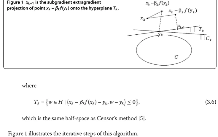
Next, we present the modified subgradient extragradient method as follows.
Algorithm .(The modified subgradient extragradient method)
Step : select an initial guessx∈Harbitrarily, setk= and construct the half-space
Ck:=w∈H|c(xk) +c(xk),w–xk≤;
Step : given the current iterationxk, compute
yk=PCk
xk–βkf(xk), (.)
where
βk=σρmk, σ> ,ρ∈(, ) (.)
andmkis the smallest nonnegative integer, such that
βkf(xk) –f(yk)+ Mβkxk–yk≤νxk–yk, (.)
whereM=MMandν∈(, ).
Step : calculate the next iterate,
xk+=PTk
Figure 1 xk+1is the subgradient extragradient
projection of pointxk–βkf(yk) onto the hyperplaneTk.
where
Tk=
w∈H|xk–βkf(xk) –yk,w–yk
≤, (.)
[image:6.595.112.480.89.320.2]which is the same half-space as Censor’s method [].
Figure illustrates the iterative steps of this algorithm.
At the end of this section, we list the alternating theorem [, ] for the solutions of
VI(C,f), whereCis given by (.). This result will be used to prove the convergence the-orem of our algorithm in the next section.
Theorem . Assume that the solution setSOL(C,f)ofVI(C,f)is nonempty.Given x∗∈C. Then x∗∈SOL(C,f)iff we have either
. f(x∗) = ,or
. x∗∈∂Cand there exists a positive constantβsuch thatf(x∗) = –βc(x∗).
4 Convergence theorem of the algorithm
In this section, we prove the weak convergence theorem for Algorithm .. First of all, we give the following lemma, which plays a crucial role in the proof of our main result.
Lemma . Let{xk}∞k=and{yk}∞k=be the two sequences generated by Algorithm..Let u∈SOL(C,f)and letβkbe selected as(.)and(.).Then,under the Conditions., . and.,we have
xk+–u≤ xk–u– –νxk–yk, ∀k≥. (.)
Proof Takingu∈SOL(C,f) arbitrarily, for allk≥, using (.) and the monotonicity of f, we have
xk+–u≤xk–βkf(yk) –u–xk–βkf(yk) –xk+
=xk–u–xk–xk++ βk
f(yk),u–xk+
=xk–u–xk–xk++ βk
f(yk) –f(u),u–yk
+f(u),u–yk+f(yk),yk–xk+
≤ xk–u–xk–xk+
+ βk
=xk–u–xk–yk–yk–xk+– xk–yk,yk–xk+
+ βk
f(u),u–yk+f(yk),yk–xk+
=xk–u–xk–yk–yk–xk+
+ xk–βkf(yk) –yk,xk+–yk
+ βk
f(u),u–yk
. (.)
By the definition ofTk, we get
xk–βkf(yk) –yk,xk+–yk
=xk–βkf(xk) –yk,xk+–yk+βk
f(xk) –f(yk),xk+–yk
≤βk
f(xk) –f(yk),xk+–yk
≤βkf(xk) –f(yk)xk+–yk. (.)
Substituting (.) into the last inequality of (.), thus we obtain
xk+–u≤ xk–u–xk–yk–yk–xk+
+ βkf(xk) –f(yk)xk+–yk
+ βk
f(u),u–yk
≤ xk–u–xk–yk+ βk
f(u),u–yk
+βkf(xk) –f(yk)
. (.)
The subsequent proof is divided into following two cases. Case :f(u)= .
Using Theorem ., there exists aβu> such thatf(u) = –βuc(u). By the subdifferential inequality, we have
c(u) +c(u),yk–u
≤c(yk), ∀k≥. (.)
Noting the fact thatc(u) = due tou∈∂C, we have
c(u),yk–u≤c(yk), ∀k≥. (.)
Since –βu< , it follows from (.) that
–βuc(u),yk–u≥–βuc(yk), ∀k≥, it implies
f(u),yk–u
≥–βuc(yk), ∀k≥
or
By the definition ofCk, we have
c(xk) +
c(xk),yk–xk
≤, ∀k≥,
using the subdifferential inequality again,
c(yk) +
c(yk),xk–yk
≤c(xk), ∀k≥.
Adding the above two inequalities, we obtain
c(yk)≤
c(yk) –c(xk),yk–xk
, ∀k≥. (.)
Combining (.) and (.), we have by using (iii) and (iv) of Condition .
f(u),u–yk≤βuc(yk)
≤βu
c(yk) –c(xk),yk–xk
≤Myk–xk, (.)
whereMis defined as before. Substituting (.) into the last inequality of (.), we obtain
xk+–u≤ xk–u–xk–yk+ Mβkyk–xk
+βkf(xk) –f(yk).
Finally, from the condition ofβkgiven by (.), we get
xk+–u≤ xk–u– –νxk–yk.
Case :f(u) = .
From (.), we can easily get
xk+–u≤ xk–u–xk–yk+βkf(xk) –f(yk). (.)
Obviously, (.) implies
βkf(xk) –f(yk)
≤νxk–yk, ν∈(, ). (.)
Thus, (.) follows from the combination of (.) and (.).
Indeed, substituting (.) into (.), we get
σρmkf(xk) –f(yk)+ Mσρmkxk–yk≤νxk–yk. (.)
Letmbe the smallest nonnegative integer, such that
whereκis the Lipschitz constant off. Noting thatf(xk) –f(yk) ≤κxk–yk, we assert from (.) and (.) thatmk≤m, which implies
βk≥σρm, (.)
namelyinfk≥{βk}> .
Theorem . Assume that Conditions.-.hold.Then the two sequences{xk}∞k=and {yk}∞
k=generated by Algorithm.converge weakly to the same point z∈SOL(C,f), fur-thermore
z= lim
k→∞PSOL(C,f)(xk). (.)
Proof By Lemma .,
xk+–u≤ xk–u
for allk≥, so there exists
a= lim
k→∞xk–u
and the sequence{xk}∞k=is bounded. From (.), we have
xk–yk≤ –ν
xk–u–xk+–u.
Hence,
xk–yk→ (k→ ∞). (.)
In addition,
f(xk) –f(yk)→ (k→ ∞).
Using the Cauchy-Schwartz inequality,
yk=yk–xk+xk ≤ yk–xk+xk,
hence, the sequence{yk}∞k=is also bounded.
Letω(xk) be the set of weak limit points of{xk}∞k=,i.e.,
ω(xk) =
z| ∃{xkj}
∞
j=⊂ {xk}∞k=s.t.xkjz
.
Since the sequence{xk}∞k=is bounded,ω(xk)=∅. Takingz∈ω(xk) arbitrarily, there ex-ists some subsequence{xkj}∞j=of{xk}∞k=, such that
Equation (.) together with (.) leads to
ykjz (j→ ∞). (.)
Due toyk∈Ckand the definition ofCk, we have
c(xk) –c(xk),xk–yk≤, (.)
then, using the Cauchy-Schwartz inequality again,
c(xk)≤c(xk)xk–yk. (.)
According to (iii) in Condition ., we can deduce thatc(x) is bounded on any bounded sets ofH, so there existsM> such thatc(xk) ≤Mfor allk≥, and then
c(xk)≤Mxk–yk → (k→ ∞). According to (ii) in Condition ., we have
c(z)≤lim inf
j→∞ c(xkj)≤. Hence,z∈C.
Now, we turn to showingz∈SOL(C,f). Define
Tv=
⎧ ⎨ ⎩
f(v) +NC(v), ifv∈C, ∅, ifv∈/C,
whereNC(v) is defined by (.). Obviously,T is a maximal monotone operator. For arbitrary (v,w)∈G(T), we have
w∈T(v) =f(v) +NC(v),
equivalently,
w–f(v)∈NC(v).
Settingy=zin (.), we get
w–f(v),z–v≤. (.)
On the other hand, by the definition ofykand (.), we have
xk–βkf(xk) –yk,yk–v≥
or
yk–xk
βk
+f(xk),v–yk
for allk≥. Using (.) and (.), we obtain
w,v–z ≥f(v),v–z
≥f(v),v–z–
yk j–xkj
βkj
+f(xkj),v–ykj
=f(v),v–ykj+ykj–z
–
y
kj–xkj
βkj
+f(xkj),v–ykj
=f(v),v–ykj
+f(v),ykj–z
–
y
kj–xkj
βkj
+f(xkj),v–ykj
=f(v) –f(ykj),v–ykj
+f(ykj) –f(xkj),v–ykj
–
yk j–xkj
βkj
,v–ykj
+f(v),ykj–z
≥f(v),ykj–z
+f(ykj) –f(xkj),v–ykj
–
yk j–xkj
βkj
,v–ykj
. (.)
By virtue of (.), (.) and Condition ., takingj→ ∞in (.), we have
w,v–z ≥. (.)
SinceT is a maximal monotone operator, (.) means that ∈T(z) and consequently z∈T–() =SOL(C,f).
Now we are in a position to verify thatxk z (k→ ∞). In fact, if there exists an-other subsequence {xki}∞i= of {xk}∞k=, such that xki z¯∈ SOL(C,f), but ¯z=z,
not-ing the fact that {xk–u}∞k= is decreasing for allu∈SOL(C,f), we obtain by using Lemma .
lim
k→∞xk–z=jlim→∞xkj–z<jlim→∞xkj–¯z = lim
k→∞xk–¯z=ilim→∞xki–¯z < lim
i→∞xki–z=klim→∞xk–z. (.) This is a contradiction, so z¯=z. Consequently, we havexk z (k→ ∞) andyk z (k→ ∞).
Finally, we show that z=limk→∞PSOL(C,f)(xk). Putuk=PSOL(C,f)(xk), using (.) again
andz∈SOL(C,f),
By Lemma ., there existsu∗∈SOL(C,f) such thatuk→u∗. Therefore, takingk→ ∞ in (.), we have
z–u∗,u∗–z≥, (.)
thereforez=u∗. The proof is complete.
5 Convergence rate of the modified method
In this section, we prove the convergence rate of our modified subgradient extragradient method in the ergodic sense. The base of the complexity proof is ([, ])
SOL(C,f) =
u∈C
z∈C|f(u),u–z≥. (.)
In order to prove the convergence rate, now we give the key inequality of our method. Indeed, by an argument very similar to the proof of Lemma ., it is not difficult to get the following result.
Lemma . Let{xk}∞k=and{yk}∞k=be the two sequences generated by Algorithm.and letβkbe selected as(.)and(.).Assume that the Conditions., .and.are satisfied. Then,for any u∈C,we have
xk+–u≤ xk–u– –νxk–yk+ βk
f(u),u–yk. (.)
Theorem . For any integer n> ,we have a zn∈H,which satisfies znz,z∈SOL(C,f) and
f(u),zn–u≤x–u
ϒn
, ∀u∈C, (.)
where
zn=
n k=βkyk
ϒn
and ϒn= n
k=
βk. (.)
Proof Using (.), we get
βk
f(u),yk–u≤ xk–u–xk+–u. (.)
Summing the inequality (.) overk= , , . . . ,n, we get
f(u), n
k= βkyk–
n
k= βku
≤ x–u, ∀u∈C.
From the notation ofϒnandznin (.), we derive
f(u),zn–u
≤x–u
ϒn
On the other hand, sinceznis a convex combination ofy,y, . . . ,yn, it is easy to see that znz∈SOL(C,f) due to the fact thatykz∈SOL(C,f) proved by Theorem .. The
proof is complete.
Letβ=σρm. From (.),β
k≥βholds for allk≥ and this together with (.) leads to
ϒn≥(n+ )β,
this means the modified subgradient extragradient method hasO(n) convergence rate. In fact, for any bounded subsetD⊂Cand given accuracy> , our algorithm achieves
f(u),zn–u≤, ∀u∈D,
in at most
n=
m β
iterations, wherezndefined in (.) andm=sup{x–u|u∈D}.
6 Results and discussion
Since the modified subgradient extragradient method proposed in this paper is relaxed and self-adaptive, it is easily implemented. A weak convergence theorem for our algorithm is proved due to the alternating theorem for the solutions of variational inequalities. Our results in this paper effectively improve the existing related results.
7 Conclusion
Although the extragradient methods and the subgradient extragradient methods have been widely studied, the existing algorithms all face the problem that the projection op-erator is hard to calculate. The problem can be solved effectively by using the modified subgradient extragradient method proposed in this paper, since two projections onto the original domain are all replaced with projections onto some half-spaces, which is very eas-ily calculated. Besides, the step size can be selected in some adaptive ways, which means that we have no need to know or to estimate the Lipschitz constant of the operator. Fur-thermore, we prove that our method hasO(n) convergence rate.
Competing interests
The authors declare that they have no competing interests.
Authors’ contributions
All authors contributed equally to the writing of this paper. All authors read and approved the final manuscript.
Acknowledgements
This work was supported by the Foundation of Tianjin Key Lab for Advanced Signal Processing (2016 ASP-TJ02).
Publisher’s Note
Springer Nature remains neutral with regard to jurisdictional claims in published maps and institutional affiliations.
References
1. Kinderlehrer, D, Stampacchia, G: An Introduction to Variational Inequalities and Their Applications. Society for Industrial and Applied Mathematics, Philadelphia (2000)
2. Korpelevich, GM: An extragradient method for finding saddle points and for other problems. Èkon. Mat. Metody12, 747-756 (1976)
3. Nadezhkina, N, Takahashi, W: Weak convergence theorem by an extragradient method for nonexpansive mappings and monotone mappings. J. Optim. Theory Appl.128, 191-201 (2006)
4. Censor, Y, Gibali, A, Reich, S: Extensions of Korpelevich’s extragradient method for the variational inequality problem in Euclidean space. Optimization61, 1119-1132 (2012)
5. Censor, Y, Gibali, A, Reich, S: The subgradient extragradient method for solving variational inequalities in Hilbert space. J. Optim. Theory Appl.148, 318-335 (2011)
6. Censor, Y, Gibali, A, Reich, S: Strong convergence of subgradient extragradient methods for the variational inequality problem in Hilbert space. Optim. Methods Softw.26, 827-845 (2011)
7. Yao, YH, Postolache, M, Liou, YC, Yao, ZS: Construction algorithms for a class of monotone variational inequalities. Optim. Lett.10, 1519-1528 (2016)
8. Yao, YH, Liou, YC, Kang, SM: Approach to common elements of variational inequality problems and fixed point problems via a relaxed extragradient method. Comput. Math. Appl.59, 3472-3480 (2010)
9. Yao, YH, Noor, MA, Liou, YC, Kang, SM: Iterative algorithms for general multivalued variational inequalities. Abstr. Appl. Anal.2012, 768272 (2012)
10. Yao, YH, Noor, MA, Liou, YC: Strong convergence of a modified extragradient method to the minimum-norm solution of variational inequalities. Abstr. Appl. Anal.2012, 817436 (2012)
11. Zegeye, H, Shahzad, N, Yao, YH: Minimum-norm solution of variational inequality and fixed point problem in Banach spaces. Optimization64, 453-471 (2015)
12. Yao, YH, Shahzad, N: Strong convergence of a proximal point algorithm with general errors. Optim. Lett.6, 621-628 (2012)
13. He, S, Yang, C: Solving the variational inequality problem defined on intersection of finite level sets. Abstr. Appl. Anal. 2013, 942315 (2013)
14. Fukushima, M: A relaxed projection method for variational inequalities. Math. Program.35, 58-70 (1986) 15. Takahashi, W: Nonlinear Functional Analysis. Yokohama Publishers, Yokohama (2000)
16. Goebel, K, Reich, S: Uniform Convexity, Hyperbolic Geometry and Non-expansive Mappings. Dekker, New York (1984) 17. Hiriart-Urruty, JB, Lemarchal, C: Fundamentals of Convex Analysis. Springer, Berlin (2001)
18. Rockafellar, RT: On the maximality of sums of nonlinear monotone operators. Trans. Am. Math. Soc.149, 75-88 (1970) 19. Opial, Z: Weak convergence of the sequence of successive approximations for nonexpansive mappings. Bull. Am.
Math. Soc.73, 591-597 (1967)
20. Takahashi, W, Toyoda, M: Weak convergence theorems for nonexpansive mappings and monotone mappings. J. Optim. Theory Appl.118, 417-428 (2003)
21. He, S, Xu, HK: Uniqueness of supporting hyperplanes and an alternative to solutions of variational inequalities. J. Glob. Optim.57, 1375-1384 (2013)
22. Nguyen, HQ, Xu, HK: The supporting hyperplane and an alternative to solutions of variational inequalities. J. Nonlinear Convex Anal.16, 2323-2331 (2015)
23. Facchinei, F, Pang, JS: Finite-Dimensional Variational Inequalities and Complementarity Problems, vols. I and II. Springer Series in Operations Research. Springer, New York (2003)
24. Cai, XJ, Gu, GY, He, BS: On theO(1
t) convergence rate of the projection and contraction methods for variational