Sabine A One Dimensional Bulk Shielding Program EUR 3636

EUR 3636e

EUROPEAN ATOMIC ENERGY COMMUNITY - EURATOM

SABINE S

A ONE DIMENSIONAL BULK

SHIELDING PROGRAM

by a p i

C. PONTI* H. PREUSCH** and H. SCHUBART***

** A.I.V. Büro Darmstadt

*** Technische Hochschule Hannover

1967

LEGAL NOTICE

This document was prepared under the sponsorship of the Commission of the European Communities.

Neither the Commission of the European Communities, its contractors nor any person acting on their behalf :

Make any warranty or representation, express or implied, with respect to the accuracy, completeness, or usefulness of the information contained in this document, or that the use of any information, apparatus, method, or process disclosed in this document may not infringe privately owned rights ; or

Assume any liability with respect to the use of, or for damages resulting from the use of any information, apparatus, method

or process disclosed in this document. , ht

This report is on sale at the addresses listed on cover page 4

at the price of FF 8.50 FB 85.— DM 6.80 Lit. 1.060 Fl. 6.20

When ordering, please quote the EUR number and the title, which are indicated on the cover of each report.

Printed by Vanmelle S.A. Brussels, October 1967

This document was reproduced on the basis of the best available copy.

EUR 3636 e

S A B I N E — A ONE DIMENSIONAL BULK SHIELDING PRO-GRAM by C. PONTI*, H. PREUSCH** and H. SCHUBART***

* Euratom

** A.I.V. Büro Darmstadt

*** Technische Hochschule Hannover

European Atomic Energy Community — EURATOM

Joint Nuclear Research Center — Ispra Establishment (Italy) Reactor Physics Department — Reactor Theory and Analysis Euratom Contract No. 149-64-11 ISPD

Brussels, October 1967 — 64 Pages — 3 Figures — FB 85

This report describes the theory and the use of a program for bulk shield design, written in Fortran IV for IBM 7090 or 360.

The removal diffusion model has been applied ; particular attention has been paid to the treatment of the removal sources in the diffusion equations.

EUR 3636 e

S A B I N E — A ONE DIMENSIONAL BULK SHIELDING PRO-GRAM by C. PONTI*, H. PREUSCH** and H. SCHUBART***

* Euratom

** A.I.V. Büro Darmstadt

*** Technische Hochschule Hannover

European Atomic Energy Community — EURATOM

Joint Nuclear Research Center — Ispra Establishment (Italy) Reactor Physics Department — Reactor Theory and Analysis Euratom Contract No. 149-64-11 ISPD

Brussels, October 1967 — 64 Pages — 3 Figures — FB 85

This report describes the theory and the use of a program for bulk shield design, written in Fortran IV for IBM 7090 or 360.

Neutron fluxes for 26 energy groups and gamma fluxes for 7 groups are calculated in plane, cylindrical and spherical geometry.

Experimentally determined removal c.s. are used for the more important shielding materials.

Gamma sources include the radiation emitted either by fission or neutron capture or inelastic neutron scattering. Three forms of region dependent build-up-factors may be used to determine the gamma fluxes : build-up-factors for 6 materials have been calculated with the BIGGI 3 gamma transport program.

Other quantities calculated by SABINE may be any neutron response function, gamma dose and energy deposition.

Neutron fluxes for 26 energy groups and gamma fluxes for 7 groups are calculated in plane, cylindrical and spherical geometry.

Experimentally determined removal c.s. are used for the more important shielding materials.

Gamma sources include the radiation emitted either by fission or neutron capture or inelastic neutron scattering. Three forms of region dependent build-up-factors may be used to determine the gamma fluxes : build-up-factors for 6 materials have been calculated with the BIGGI 3 gamma transport program.

EUR 3636e

EUROPEAN ATOMIC ENERGY COMMUNITY - EURATOM

SABINE

A ONE DIMENSIONAL BULK

SHIELDING PROGRAM

by

C. PONTI*, H. PREUSCH** and H. SCHUBART***

** A.I.V. Büro Darmstadt

*** Technische Hochschule Hannover

1967

SUMMARY

This report describes the theory and the use of a program for bulk shield design, written in Fortran IV for IBM 7090 or 360.

The removal diffusion model has been applied ; particular attention has been paid to the treatment of the removal sources in the diffusion equations.

Neutron fluxes for 26 energy groups and gamma fluxes for 7 groups are calculated in plane, cylindrical and spherical geometry.

Experimentally determined removal c.s. are used for the more important shielding materials.

Gamma sources include the radiation emitted either by fission or neutron capture or inelastic neutron scattering. Three forms of region dependent build-up-factors may be used to determine the gamma fluxes : build-up-factors for 6 materials have been calculated with the BIGGI 3 gamma transport program.

Other quantities calculated by SABINE may be any neutron response function, gamma dose and energy deposition.

KEYWORDS

F-CODES

PROGRAMMING SHIELDING DIFFUSION

DIFFERENTIAL EQUATIONS NEUTRON FLUX

GAMMA RADIATION SHIELDING MATERIALS BUILDUP

S-CODES

CONTENTS

Introduction 5

1. Definition of the Problem 7 1.1 Source of Radiation 7

1.2 Geometry 7 1.3 The Shield Regions 11

2. Calculation of the Neutron Flux 12 2.1 Neutron Energy Group Structure 12 2.2 The Source Distribution for Removal Neutrons 1^

2. 2.1 Plane Geometry 12*

2. 2. 2 Cylindrical Geometry 15 2.2.3 Spherical Geometry 16 2.2.4 "Disk" Geometry 16 2.3 Removal Flux Calculation 17

2.4 The Source Terms of the Diffusion Equations 18

2.5 Group Cross-Sections Library 21 2.5.1 Data for the Removal Flux Calculation 21

2.5.2 Data for the Diffusion Calculation 21

2.6 Solution of the Diffusion Equation

2h

2.7 Boundary Conditions 26 2.7.1 Outer Boundary 26 2.7.2 Inner Boundary 26

2.8 Air Gaps 27 2. 8.1 P1 Approximation 27

2.8.2 A Different Optional Treatment 28

2.9 Response Functions 28

3. Calculation of the Gamma Flux 30

4

-3.2.1 Sources inside the Core 31

3. 2. 2 Sources inside the Shield 33

3. 3 Calculation of the Gamma Fluxes 3^

3.4 Build-up-Factors 3**

3.5 Gamma Energy Deposition 38

3. 6 The Numerical I n t e g r a t i o n s 38

3.7 Gamma Data Library

ko

4. U s e r ' s Manual ^2

4.1 Computer Requirements ^2

4.2 Input Specifications ^2

4.3 Choice of Mesh Intervals 52

4.4 Output of the Program 5^

Conclusion 55

Acknowledgements 56

References 57

APPENDICES

A. The Factorization of the Diffusion Equation 59

B. The Solution of the System of Differential

5

-S A B I N E

A ONE DIMENSIONAL BULK SHIELDING PROGRAM1*'

INTRODUCTION

This report describes the physical foundations, the mathe-matical methods, the structure and the use of the program

Sabine.

The code is the result of an effort of formulating and applying the Removai-Diffusion model in a way as accurate as possible, of solving a wide class of shielding problems, taking into account several possible geometries of the

source and of the shielding regions, and of providing the maximum amount of information concerning neutron and gamma

penetration, heat deposition, or reaction rates.

The Removal-Diffusion model is a way of solving neutron penetration problems suggested about ten years ago [ï]: it has been applied with more or less refiniments in several programs for shielding calculations [2, 3> 43. On the

ba-sis of the experience made up to now on these programs, the authors think that this method of solution is satisfac-tory and efficient, at least when applied to massive hydro-geneous shields, and that the recourse to more sophisticated methods, does not give generally an increase in accuracy

such as to compensate for the greater cost.

An experimental program of removal c. s. measurements, develo-ped in connection with the Padova University C53, has provi-ded the basic data; on the other hand special care was ta-ken for applying the Removal-Diffusion method in a way as coherent and general as possible.

SABINE is a Fortran IV program for IBM 7090 or 360. It calculates the following quantities as functions of the distance from the core boundary:

a) Neutron fluxes for up to 35 groups b). Total neutron dose rate

c) An integral over energy of the total neutron flux times

6

-an a r b i t r a r y response function, e.g. r e a c t i o n r a t e ,

a c t i v a t i o n , e t c .

d) Gamma fluxes for up to 7 energy groups, s e p a r a t i n g the

c o n t r i b u t i o n s of the d i f f e r e n t source r e g i o n s .

e) Gamma h e a t i n g and dose r a t e .

The gamma flux i s obtained as the product of the u n c o l l i

-ded flux times a region dependent b u i l d - u p - f a c t o r , which

i s i n t e r p o l a t e d from a proper t a b l e of v a l u e s . Tables of

b u i l d - u p - f a c t o r s for several m a t e r i a l s and gamma groups

have been c a l c u l a t e d by the BIGGI 3 [6} gamma t r a n s p o r t

code.

The development of the program SABINE has been the object

of a c o l l a b o r a t i o n between the Shielding Group of

EURATOM-I s p r a , the A.E.G. Kernenergieanlagen i n Frankfurt/Main, the

A.I.V. BÜRO i n Darmstadt, and the "Arbeitsgruppe für

bautechnischen Strahlenschutz der T.H.Hannover".

7

-DEFINITION OF THE PROBLEM. 1.1 Sources of Radiation

The program SABINE determines the energy dependent neutron and gamma fluxes through a shield assembly composed of 1 to 20 homogeneous regions, which surround a source (core) composed of two regions.

The neutron source is a fission density distribution inside the 2 core regions; the gamma source is the sum of 3 terms: a) gamma radiation emitted by fission and fission products

at equilibrium,

b) neutron capture gamma rays,

c) radiation from inelastic neutron scattering.

In the core regions the gamma source may take into account all the 3 terms; in the shield, only items b and c are considered.

1.2 Geometry

The geometry of the core is defined by an index IGRC which may take four values, corresponding to the following possi-bilities:

Table 1

IGRC Geometry of the core 0 Infinite plane slab

1 Finite or infinite cylinder radiating in radial direction

2 Sphere

8

-In the different cases, the two core regions may be respec-tively: 2 plane slabs, a cylinder surrounded by a coaxial cylindrical annulus of equal or unequal height, a sphere surrounded by a spherical shell, two coaxial oylinders with equal or unequal radii (Fig.1). This last case is for

instance that of the axial shield of a cylindrical reactor. A particular feature of the SABINE program is that the

geometry of the shield can be approximated in different ways for the different calculations to be performed. This

fact has mainly two reasons: with the aim of saving ma-chine time, the real geometry can be approximated with a simpler one for a particular type of calculation for whioh this implies tolerable errors; furthermore, if our inte-rest is focused over a given quantity or region of the assembly, we can choose the geometrical representation which is more convenient for that.

In what follows we will oall "primary gamma" the radiation originated from sources inside the core, and "secondary gamma" the radiation produced by the gamma sources inside

the shield; besides we note that in the frame of our mo-del, the primary gamma flux and the removal neutron flux obey to equations which are formally equal.

The shield geometry for the different possible oaloula-tions is defined by the following indexes:

IGRS: for the Removal neutrons and primary gamma fluxes IGDS: for the solution of the Diffusion equation

IGSS: for the calculation of the Secondary gamma fluxes. These indexes may take the values:

0 : the shield regions are plane slabs

1 : the shield regions are cylindrical annuii 2 : the shield regions are spherioal shells

^ J i J i

IGRC« O IGRCs 1

IGRC ζ 2 IGRCr 3

10

their axis, similarly to the case IGRC=3 (Pig. 1 ) ; this situation will be called briefly "disk" geometry. Most of the running time needed by SABINE is spent in calcula­ ting the removal neutron fluxes and the gamma fluxes, and these calculations are more time consuming for spherical and mainly for cylindrical geometry: when possible the indexes IGRS=0 and IGSS=0 or 3 should be preferred.

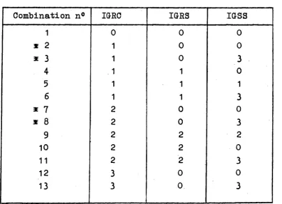
Table 2 summarizes the possible combinations of the geome­ trical indexes; the index IGDS is not dependent upon the others, and may be quite arbitrary. It happens frequently that one has to solve problems for which a "disk" geometry is preferable for the removal flux calculation and a sphe­ rical geometry for the solution of the diffusion equation.

11

In the cases indicated with x, the outer surface of the

core and the inner surface of the shield are not coincident, but only tangent in one point or one linet the space between them is assumed to be filled with the material of the first shielding region, but no gamma sources are considered there.

1.3 The'Shield Regions

12

2. CALCULATION OF THE NEUTRON FLUX. 2.1 Neutron Energy Group Structure

In what follows reference is made for sake of simplicity to the group structure of the neutron data library prepa-red for SABINE, that is presently in use; however the ar-guments can be easily generalized for a different choice of the energy groups.

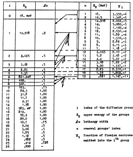
The energy limits as well as other details concerning the neutron groups are given in Table 3.

The energy range between 0.5 and 18 Mev has been divided into 19 removal groups, having roughly constant energy width;'the calculation of the total neutron flux is per-formed in a 26 groups scheme, that covers the energy range between 0 and about 15 Mev, with lethargy intervals of 0.5 - 1.,The number of these groups and their energy range have been chosen mainly on the basis of the following conside-rations:

1) The slowing down length of each group must be smaller than the relaxation length of the penetrating component, described by the removal flux.

2) The energy width of the groups should be narrow enough, in order that the dependence of the group averaged c.s. upon the weighting spectrum be not important.

3) The lethargy mesh should be more fine in the fast region than elsewhere because: a) this is the most important part of the spectrum to be determined; b) it is general-ly the most penetrating component; c) the presence of the inelastic scattering implies a detailed treatment of the transfer matrix.

4) The running time for the calculation of the neutron diffusion and slowing down in SABINE, using the maximum number of groups ,35, allowed by the program, is about

cal-13

TABLE 3

Energy Structure of the Neutron Groups in the Present Library

i 0 1 2

3

4

δ

9

18. NeV

14.918 6.065 3.66 2.23 1.35 821.keV 49b. 302. 11*3. 86.5 31.8 11.7 4.31 1.58 583. eV 214. 78.9 29.0 10.7 5.04 3.06 1.85 1.12 .682 .414 .200 Ju .9 .5 .5 .5 .5

.5

.5

.5

.75

.75

.5

.5

.5

.5

.5

f

■ y

s

f

À

M

/M

/ /

i

V

Γ

ΙΑ

Χ

prr

7

/

i

¥

à

5

8

9

■ W

19 Β,, (MeV) 18. 16.5 14.918 14. 13. 12. 11. 10. 9. 8. 7. 6.065 5.2 4.4 3.68 3.00 2.33

1.55

index of the diffusion group

„ upper energy of the groups

u lethargy width

removal groups' index

fraotion of fission neutrons th

14

-culation, in plane geometry, and smaller for cylindrical

and spherical geometry, and hence reducing the number of

groups does not mean, in general, an important saving.

The upper limit of the highest energy group has been cho­

sen higher than necessary: it could be reduced, but not

too much if one is interested in the knowledge of the

fast spectrum.

2. 2 The Source Distribution for Removal Neutrons

The program considers as neutron sources the fission neu­

trons generated inside region 1 and 2. For both of these

regions the program computes the number of neutrons S (Q)

emitted with energy corresponding to the removal group n,

per unit volume and time at the point Q, as

S

($) = SoX

-vF(Q)

Sb = fission density at the outer edge of the region

(fissions/cm .sec)

Y th

_{An = fraction of fission neutrons released in the n}

group according to the Cranberg fission spectrum.

V = average number of neutrons per fission = 2.46

P(Q)= function describing the space dependence of the fis­

sion density in the region considered.

Por the different possible geometries of the source regions

(cfr. section 1.2 and Pig. 1), P(Q) may have the different

forms considered in the following.

2.2.1 Plane Geometry, IGRC=0

In this case the function depends upon one variable z* ;

P(Q)=P(z'). The z'-axis has the origin on the outer face of

the region and is oriented towards the inner of the region:

we have for instance (see Pig.1)

in region 1 zi = t. -Ζ (la)

15

-F(z*) must be normalized in such a way to have the value

1 on the outer boundary of the region: F(0)=1.

The function P(z') may be specified in two ways:

a) pointwise, that is providing (M+1) values P

at

equidistant points:

F

m=

(

'

'

m

"

>H~ >

1.2,...,M+1

where t is the thickness of the region.

Necessarily

P

1 and M ^ 50

In this case the program computes the J coefficients

of the polynomial of degree (J-1) which best fits,

in the least squares sense, the given space

distri-bution.

F(*')*^»i

"

(2)

A value for J<10 must be precised by the user.

b) the J coefficients of the polynomial can be given

as input data: also in this case J^ 10 and a.= 1

(P(0)=

=1).

2.2.2 Cylindrical Geometry, IGRC=1

We assume in this case

P(Q)= h(r»).g(z)

In region 1 and 2 we have respectively (see Pig.1)

r2 = ti+'fc2~r ^

16 ­

a.(a.=l) or providing a table of values g_=g(z ) wi

_{t h}

z

= (m­l)lj2M, m =1, 2 , . . . ,Μ+1, M 50, g

1,

The f u n c t i o n h ( r ' ) may take one of the forms:

h ( r ' ) = e­*

"

(

)

h ( r ' ) = ¿ b

r · ^ "

,

b.=1 , J < 10

(

)

j¿i

If the form (4a) i s chosen, the value of k has to be given;

i f the form (4b) i s chosen, the user has to provide the

c o e f f i c i e n t s b ., or a s e t of values h. =h(r_·)·, f o r M+1

e q u i d i s t a n t r a d i a l p o i n t s , with r!=0 (outer s u r f a c e ) ,

Γ

Μ+1

*

surface, and h..=1: i n t h i s case the

c o e f f i c i e n t s b . are calculated by the program.

J

2. 2. 3 Spherical Geometry, IGRC=2

In t h i s case the souroe d i s t r i b u t i o n i s again a function

h ( r ' ) ; r ' has the form (3) and h ( r ' ) has the same form,

d e s c r i p t i o n and l i m i t a t i o n s as the corresponding function

in c y l i n d r i c a l geometry.

2.2.4 Disk Geometry, IGRC=3

As explained i n section 1.2, t h i s expression means t h a t

the source regions c o n s i s t of two c y l i n d e r s which are

shielded i n the d i r e c t i o n of t h e i r a x i s ; i n t h i s oase the

d i s t r i b u t i o n function i s

P(Q)= h ( r ) g ( z ' )

r is the distance of the point Q from the ζ axis, and z' is

the distance between Q and the right boundary of the region as in (1)„

17

2.3 Removal Flux Calculation

The removal flux is calculated (see for instance ref. 1)

as the flux of neutrons which have not suffered "removal"

collisions.

For each of the 19 groups the contribution to the removal

flux in a point P, due to a differential volume element

dV around the source point Q (for isotropic source) is

apr

s(q)K(p

Q)

47Γ pi$

where

S(Q) = source strength in Q for the group considered

(neutron/cm

sec)

K(P,Q)=: exp[­| £.

(s)ds]

•¿

= region dependent macroscopic removal c.s.

The removal flux in Ρ is the result of the integration of

eq.(5) over the source volume: this is a numerical inte­

gration which is performed as reported in Part 3· The point

Ρ may move along the r or ζ axis shown in Fig. 1 for the

possible geometries.

After the removal fluxes and the removal collision densities,

have been calculated for each of the 19 groups of Table 3,

namely

F*(P) and F 5

Σ1

(Ρ), η ­ 1,2',... 19

these are added to get removal fluxes and collision densi­

ties corresponding to the broad groups i.

For instance for the group i=2 one has

R. flUX

Φ ; ( Ρ ) = £

η > )

R. collision dens.

C[

(P) ~ ¿ ~

f\

( Ρ )

(

)

18

2.4 The Source Terms of the Diffusion Equations.

The coupling of the removal neutrons into the diffusion

equations, through the source terms, has to be considered

carefully when applying the R. D. (Removal Diffusion) mo­

del, especially if one wishes to get from this simple

description of the physical reality a good estimate of

the neutron spectrum.

On one side we have a R. flux describing the fast neutron

penetration- which strictly refers to the empirical idea

of R. c. s. , and on the other the set of multigroup eqs.

that describe the neutron diffusion and slowing down,

within the frame of the D. approximation. The slowing down

of neutrons should be accounted for through a proper

transfer matrix: the same matrix will be used either for

the R or for the D neutrons, despite of the fact that their

spectra are in general different; however they should not

be so much different as to produce important deviations

in the average of the c. s. over the energy interval of the

same group. As shown in table 3 the lethargy width of the

fast groups is about 0.5.

The calculation of the total transfer matrix will be consi­

dered later: it will require some particular remarks, when

applied to the R. flux. The following notation is used:

0? (z) removal flux of group i at the point ζ

cf (z) removal collision density for the group i at ζ

£^ macroscopio absorption o. s. of the i group

XL . macroscopic total transfer c.s. from

the

i to

« th

the j energy group.

19 ­

0? (ζ) ΣΙ? are absorbed

0* (ζ) ZI* enter as diffusion neutrons into the i group (the meaning of the χ is explained below)

0\ ( z ) ^±j go into the jt h group U > i )

0f (z)£lf=cf(z)are removed from the group i.

It is clear that the sum the first three terms, which gives the total number of neutrons removed from group i (per unit volume and time at z) must be equal to cf (z), otherwise the neutron balance is not saved.

This remark may seem to be obvious, but if we think that on one side the absorption and transfer c. s. are calcula­ ted from the basic c.s. under given assumptions for the elastic and inelastic scattering, and on the other side the R.o;s. is obtained largely, on an empirical basis, with arguments quite indipendent from those which determine, the calculation of the other c. s., then we realise that generally the neutron balance is not automaticly respected, but must be explicitly imposed. The sum Σ*. + ZL. . + ZL. .¡ ...+··· is the'total, and not the removal c.s. This discrepancy is originated from ,the fact that the calculation of the transfer c.s., takes into account as usual, the elastic and inelastic scattering, and impliedly accounts also for those colli­

sions (which do not produce important energy loss or angu­ lar deflections) entering the term ZL.., which do not re­ move actually the neutron from the virgin beam.

•

In order to be coherent with the assumptions of the model, a new set of diagonal terms ¿­. . of the transfer matrix will be calculated, imposing that the balance of the re­ moved neutrons be saved, namely:

or

­ 20 ­

The other (non­diagonal) terms of the transfer matrix ac­

counting for collisions that imply important energy losses,

will be calculated in the usual way (section 2.5.2).

The sum of the terms enclosed in parenthesis in (6) will

be indicated with 2I°

because it accounts for all those

collisions which produce the loss of a neutron from the

. th

ι

energy group.

It is now possible to write the source terms of the dif­

fusion equations, considering all possible neutron transfer

as indicated in Table 3; the assumption is made that in the

"zero" group (above

~ 15 Mev) there are only removal neu­

trons, and these may be scattered only into the first group.

The source term of the first diffusion equation will hence

be:

»,<.>­o

0

*<.>­£ # . ) < ( . > < ,

(7)

The solution of this equation will be

0Λζ),

that is the

diffusion flux of the first group and

0

(ζ)=0Λζ)+0Λζ)

will be the total flux of the group.

Similarly for the following groups one has (omitting the

space dependence):

s

=

0

Σ ^

øl Σ*

3 3 = ^ 3 + ^ 3 + 0 ^

'

6

*1 ^ 1 ,

Ó*2 ^2

, 6

'

· · ·

&>

^ , 6

*6 ^ 6 6

From the 7

group on, that is below about 0.5 Mev, the

R. flux is neglected:

- 21

-2.5 Group Cross-Sections Library

2.5.1 Data for the Removal Flux Calculation

These are of two kinds: the fission neutrons spectrum and the energy dependent removal c.s.

The fraction of fission neutrons emitted in the n removal group has heen calculated on the basis of the Cranberg fis­

sion spectrum, and are written in Table 3.

The energy dependent removal c. s. come from different sour­ ces of information: if available, measured values have been chosen, as for HpO, Pb, C, Pe and. Al, which have been measu­ red at the 5,5 Mev accelerator of Padova [53, where other measurements for different materials are foreseen in the next future. These data will be included in the library as

soon as they will become" available. For the other elements or isotopes the compilations of Greenborg C73 and Avery C23 have been used.

2.5.2 Data for the Diffusion Calculation

The following microscopic group c.s. are needed for the diffusion calculation:

(τ0 absorption c.s. for the "zero" group to be put into

eq. (7)

"J-In 4 " Τ Ί

6. . t o t a l t r a n s f e r c . s . from the i to the J group. <>?u t h i s c . s . accounts f o r a l l the c o l l i s i o n s t h a t

remo-ve the neutron from the i group e i t h e r by slowing down or by absorption; i t i s 6*°u = β. ° - 6. . .

Χ Χ Χ ψ X

i>. t r a n s p o r t c. s. of the i group.

- 22

in the B-3 approximation, and GATHER the thermal spectrum in the B-1 approximation, for an homogeneous medium. Group (either micro or macro-scopic) c.s. are then averaged over the calculated (or optionally provided as input) fast and thermal spectra.

The elastic scattering kernels are correct to sixth order for anisotropic scattering in the C-M system; inelastic scattering is assumed to be isotropic in the L-system. The energy degradation by inelastic scattering is calculated considering the excitation energies when these are known, or using the evaporation model when they are not known. Further details are to be found in {9,103. As pointed ομΐ in section 2.1 the energy width of the groups is narrow enough, so that the group averaged c. s. do not strongly depend on the spectrum; for the c. s. of many elements this has been checked, but nevertheless exceptions to this rule are possible. The weighting spectrum used hitherto is the slowing-down spectrum due to a fission source in water. Other data can be added to the library for the same or different elements using an arbitrary weighting spectrum. The program SABLIB has been prepared to read the data pun­ ched by GGC, to rearrange them, to read some other libra­ ry data (e.g. the removal c.s.) and to write them on the Library Tape for SABINE.

Data for the 37 "elements" listed in Table 4 are now availa­ ble for the energy group structure of Table 3. Data for

23

Table 4

24

2. 6 Solution of the Diffusion Equation

Once the removal flux has been calculated, the program computes the source terms of the multigroup diffusion equations as explained in section 2.4. Then for each neu­ tron group i, we have to solve an equation of the fol­ lowing kind

D [jZf"(r)+ f j*'(r)î­£0(r)+S(r)«O (8) D is the diffusion coefficient calculated as 1/3Σ1

£ = ZLout+DB ,B is the buckling to account roughly for a

possible transversal leakage

¿: rand ZL° are evaluated for any group and region from

the microscopic c. s. of the elements which are present in the region: the microscopic c.s. are considered in section 2.5.2

Ρ is a geometry index (the same as IGDS in seotion 1.2) P sa 0 means plane geometry

Ρ « 1 means cylindrical geometry Ρ = 2 means spherical geometry

One has to find the solution of eq. (8) satisfying the following boundary conditions:

Β.ΟΤ)0,+Β..0+&2 = 0 at the inner boundary (8a)

boDØ'+b.jØ+bp = 0 at the outer boundary (8b) Continuity of flux and current through the internal

boundaries is assumed.

­ 25 ­

Ψ

.

f

-

ψ

-

Ζ

(9a)

v

' =

( ­ D ­ ­ T ­ )

(9b)

DØ'+UØ+V = 0

(9c)

This system has several advantages: the function U(r) can

be easily solved from eq. (9a) and inserted into (9b),

which is a linear first order differential equation sol­

vable through standard formulas; the functions U and V

can then be put into (9c) which is similarly solved for

0(r); the continuity conditions for flux and current are

easily satisfied by imposing continuity to the functions

U(r), V(r) and 0(r), as it is shown by eq. (9o); the

boundary oonditions expressed in general form by eqs.

(8a) and (8b), are easily converted into boundary condi­

tions for the functions U,V and

0

because (8a) and (8b)

are formally similar to (9c).

Actually the outer boundary condition is satisfied if

we put:

U(R )= bVboi at the outer boundary

(io)

V(R

)= bg/boJ R

of the shield

With this starting values for the functions U(r) and V(r),

the eqs. (9a and b), can be integrated (Appendix B) pro­

ceeding from outside to inside: once the values U(R

) and

V(Rj) at the inner boundary of the shield are known the

quantity:

a„­a

V(R.)

«h) "

«fwvi

(11)

is taken as inner boundary value for the function

0(r)

(see below), then eq. (9c) is integrated proceeding from

inside to outside, as shown in Appendix B.

­ 26

2.7 Boundary Conditions

It is useful to make a few more remarks about this subjeot. The user has to provide a proper set of coefficients a0,

a., up and b.., b« to represent the particular boundary conditions of his problems.

2.7.1 Outer Boundary

The coefficient b0 is not allowed to be zero (that would

produce non limited values of U and V in eq. 10), so that it has been fixed once for ever b0=1 ; only b.. and bp need

to be specified to the program. As a consequenoe of that, it is not allowed to specify the outer value of the flux (which is assumed to be a result and not a datum of the problem). The usual condition at the outer boundary is of zero incoming current, that is

J_

-

-f

+

Ψ

- °

and this corresponds to the choice b ^ , 5 , bp=0, (b0=l).

Similarly a linear extrapolation distance d= ·?£ i s

expressed by b..=D/ä, bp=0, being D the diffusion coef­ ficient of the external region.

2.7.2 Inner Boundary

Hera are a few examples of inner boundary conditions. If one needs to define a boundary value of the flux

a0= 0

0(Ri)= 0O, then the set a..= ­1

a

=

0

27 ­

^ ' ( R j ^ ) ^

w i t h

a

= 1 , a

0 , a

=0

or ­XØ'iR^JsJo w i t h

a

= 1 , a ^ O , a

=J

A l l the above boundary c o n d i t i o n s are a p p l i e d to the

d i f f u s i o n

f l u x , t h a t i s to the s o l u t i o n of the

d i f f u s i o n eq. ; and hence i n those n e u t r o n groups (1 to 6

f o r t h e scheme of Table 3) where a D. f l u x and a R. f l u x

c o h a b i t , the t o t a l f l u x w i l l s a t i s f y d i f f e r e n t boundary

c o n d i t i o n s . The only e x c e p t i o n to t h i s r u l e i s the case

a

=0, which corresponds to a given boundary value of t h e

f l u x : i n t h i s case the program t r e a t s , i t a s a t o t a l f l u x ;

t h e boundary v a l u e f o r the D. f l u x i s given i n such a c a ­

se e i t h e r by t h e d i f f e r e n c e t o t a l f l u x minus the computed

v a l u e of the R. f l u x a t the boundary, or i t i s s e t equal

zero if Übe d i f f e r e n c e were n e g a t i v e .

2.8 Air Gaps

SABINE can take account of the effect of air gaps inside

the shield through proper conditions conneotig the va­

lues of flux and current on the two sides of the gap. Let

r

, Γρ be the position coordinates and J

, J

ρ the values

of the net current at each side of the gap: J(r)= ­D0'(r) .

Two different treatments of the gap are allowed.

2. 8.1 P1 approximation

If the thickness of the gap is small compared to its

transversal dimensions, and hence the transversal leakage

is negligible, then the P1 approximation C u ] states the

following equations for the flux and current through the

gap:

'i ■

(ÜJ

J.

(12a)

01

0o

28

where fp(q) i s a function depending on the geometry:

for plane geom. (P=1) f

(q)= 1

for cylindrical geom. (P=2) f

(q)= | [

°

· +fl-q

J

for spherical geom. (P=3) f

(q)= 1 - O - q

)

'

Note that in the f i r s t case flux and current are continuous

through the gap.

,2^8.2 A Different (Optional) Treatment

If the a i r gap i s thick, r e l a t i o n s different from (12) may

be required in order, for instance, to take into account

the transversal leakage in plane or cylindrical geometry.

SABINE can take account of discontinuity conditions for

flux and current through that region, in the form

0

= * # !

'>

*

2

A

1

J

M °

In this case the user has to provide a couple of values oc

and y3 for each neutron group.

The presenoe of gaps in the problem to be solved is subjeot to two restrictions: namely the first and the last region of the shield cannot be air gaps, and two gaps cannot be side by side. No more than 3 gaps of this type may be pre-sent.

2.9 Response Functions

SABINE can optionally evaluate three kinds of Response functions.

a) R M - ^ ^ W f t ,; i ¿ ^ s ^ e (13)

29

This is the integral over energy of the total neutron flux times an arbitrary function of energy, which has to be specified group-wise. In this way the program can provide for instance dose rates, reaction rates, fast or epithermal flux (fj=1 for the proper groups) and so on.

b) The response function f. may be region dependent (such as that required to evaluate for instance heat deposi­ tion or activation): in this case the user has to pro­ vide a table of values for each region; then SABINE computes the function (13) inserting for fj the table of the region to which χ belongs.

o) A third possibility has been devised to calculate the reaction rate of threshold detectors. These are at pre­ sent the tool most frequently applied to get information on the fast region of the neutron spectrum.

Macroscopic c.s. for such detectors may be provided for each of the removal groups, that are finer than the diffusion ones.(see Table 3). The program itself calcu­ lates the broad group c.s., by averaging over the com­ puted removal spectrum: for any region R

V ' th x- is the (input) value for the c.s. in the η remo-*

val group;

0 ? ( * R ) , n=1,2,...19 is the removal spectrum in the middle point of the R region.

The sums are extended to those fine groups which lie in­ side the broad group i(i=1,2',... 6)

Then at any point χ belonging to region R the program evaluates

30

-3. CALCULATION OP THE GAMMA FLUXES. 3. 1 Group Structure

SABINE can compute the space distribution of the gamma fluxes for 7 energy groups. This number is practically fixed by the gamma data library which is used: to change this number (or the number of neutron groups) a new li-brary needs to be provided. The lili-brary presently in use implies the seven groups scheme shown in table 5. The

subscript g, g=1 to 7, will be used to denote gamma ener-gy groups.

Table 5

Gamma group

1 2 3 4 5 6 7

Energy limits (Mev)

0. - 1.0 1.0 - 2.0 2.0 - 3.0 3.0 - 5.0 5.0 - 7.0 7.0 - 8.5 8.5 - 10.0

3.2 Gamma Sources

Inside the core regions, namely regions 1 and 2 three kinds of sources may be considered:

a) Gamma rays from fission b) Capture gamma rays

­ 31 ­

Item a) inoludes prompt gammas emitted by fission and gam­

ma radiation by equilibrium fission products.

In the shielding regions (region 3 and following) only

sources of type b) and c) are considered.

3. 2.1 Gamma Sources Inside the Core

The gamma source for the g

group (energy emitted in form

of photons with energy belonging to the g

interval) at

the point Q of a core region is given by

S„(Q)= S

_G(Q)

Mev/cmr.sec

g »g

S

is the value of the source at the outer boundary of

»g

the region considered

G(Q) is the dimensionless function describing the space

behaviour of the source (the same for all groups),to

be described in input with the same rules and restric­

tions as for the function

FÍO) (section 2.2) describing the fission density.

If the gamma source is essentially a fission source, then

F(Q)

Oí

G(Q), and the same input information may be repea­

ted for both functions.

S

is calculated by the program as

'

26

H

■•-.¿■■•Via'·.! ν

+

δ ' · ·

Λ

· «

( u )

where

S

= boundary value of the fission density (section 2.2)

f = energy emitted by fission, and equilibrium fission

products, in the g

group (Mev/fission)

0o4=

total neutron flux of the i

group at the outer core

'A

boundary;

32

p

=£

\*.,±1*'ϊΚ

^Ώ π

(

»ìf) = microscopie (η,#) c . s . of the i

n e u t r o n group

t h

and e

element ( b a r n s )

th

'

C. _,

c a p t u r e gamma spectrum of the e

element, i . e .

'δ th

gamma energy yield in the g group per neutron capture (Mev/capture)

Ne = nuclear density of the e element in the re­

gion considered (nuclei/barn, cm) M

1i,g

£

e

e

'

e

' 3»«>

jo e

6 (i,i+j)=micro. inelastic transfer c.s. from group i to

1 T.

i+j (barns) for the e element

Q0(i»D»g)= gamma energy emitted into the g_> group, as a

result of the inelastic scattering of a neu­ tron from group i to i+j, by the e element. The sums over e include all the elements of the region; the sum over j extends to a proper number of lower groups: in the present library M=7. The second sum in (14) extends

to those neutron groups, from the L on which lie above 0.5 Mev: at present N=6; if L > N this sum is negleoted. For normal calculations it should be L=1, to account for all possible gamma sources; but if only low energy groups need to be considered, then a suitable value of L should be chosen; for instance if the inelastic scattering gammas are negligible, and only thermal neutron capture needs to be considered, set L=26. Finally if L > 2 6 no gamma source and no gamma flux is computed, and the calculation stops after the neutron results have been printed.

Formula (14) holds for region 1 and 2 but with some minor differences: in the second region it is exactly applied; in the first region the gamma source is evaluated only if S0 (fission density at the outer boundary of the region)

is positive; if S0=0, no gamma source is considered within

33

normal shielding region (but in plane geometry its présen­ os is neglected).

3.2.2 Gamma Sources Inside the Shield

In any of the shielding regions except possible air gaps, SABINE calculates the gamma source distribution in a num­ ber of points specified by the input data and then fits this distribution with the product of an exponential

function, orossing the end­point values, and a polynomial with a number of coefficients NGCF (and degree NGCF­1) to be specified in input.

The gamma source vs. the distance x1 from the core bounda­

+Vi

ry for the g group is

26 N

Λ

ν

£*ι<*ι*±,

&*±<*ι>«±,β

In plane or spherical geometry, where S is a function of one space variable (IGSS is equal zero and two respecti­ vely), the source is given by (15). In the case of cylin­ drical (IGSS=1) or disk geometry (IGSS=3), S^ is depending

g

upon one more variable X2 (along the transversal direction),

indicated by ζ or r for the cylindrical or disk geometry respectively in Pig. 1. In such cases the program assumes

v v y - v*i

)f<x

2>

f(Xp) i s assumed to be a polynomial with c o e f f i c i e n t s g i ­

ven i n i n p u t :

NCP

f(X

)=

Z^

β

χ | "

a

1

NCFé 6

34

3.3 Calculation of the Gamma Fluxes

Once the distributions of the sources for the different groups have been calculated, the program computes and prints for each required point Ρ (of the shield) and each

Οι

region r, the gamma flux G ~(P) (Mev/cm sec) due to the

th r» o 4.­Ú

sources of the g

group, contained i n the r

r e g i o n :

Γ

Β J P Q ) e x p ( ­ T : ( P Q ) )

r» e J g /iir T5ñ¿

V

r

S_(Q) = gamma energy emitted into the g group per

e> / / 3 \

unit volume at Q (Mev/cm sec)

B (PQ) = Build­up factor (see seotion 3.4), dimensionless.

χ (PQ) = ƒ ds AA^(S)

^ t k -1

AA. = l i n e a r attenuation c o e f f i c i e n t of g

group (cm )

dV(Q) = volume element around Q, which moves to cover

the whole volume V of the r · region.

The following sections explain how the B u i l d - u p - f a c t o r s

are c a l c u l a t e d and how the numerical i n t e g r a t i o n of (16)

i s worked out.

3.4 Build-up-Factors

The gamma p a r t of the data l i b r a r y of SABINE i n c l u d e s , f o r

each gamma group, a t a b l e of "point i s o t r o p i c dose B u i l d ­

up-Factors" vs. 1he distance t ( i n m . f . p . ) from the source

point Q to the dose point P, for seven m a t e r i a l s (see Ta­

ble 6) ranging from a i r to lead.

All what follows r e f e r s to each of the gamma groups; the

s u b s c r i p t g w i l l be omitted for sake of s i m p l i c i t y .

35 ­

Now assume we need to calculate the B. u. F. to be inserted

in eq. (16), for a laminated medium such as shown in Fig.2:

let Q be a point souroe in region 1 containing the mate­

rial 1, and Ρ the dose point in the Ν

region containing

+Vi

the Ν

material, x

the part of segment PQ inside region

η with linear attenuation coefficient

μ,

/v

. Now let

*1

Λ

ι

*2 " *1

Λ>

2

*N

*N-1

/ V N

One can choose now among three different ways of calcula­

ting the B.u.F. vs. t, namely B(t), which provide the sa­

me result if the path t lies within a single region, but

different results in a laminated medium (Fig. 3). The user

may choose which way he needs by specifying the proper in­

put value NBU:

NBU « 1

B(t

) = % ( t

)

The B. u. F. is calculated by interpolation between the

values tabulated for the material of the region to which

the dose point Ρ belongs.

NBU = 2

The calculation is done with the Broder' s fl4j

formula

Ν

Ν

B(t„) = £

B

(t_) - f

B (t

J

Ν n=1 η η n=¿ η η­1

which is easier to understand in the following

recurrent form:

Β ( ^ )

m

B^t

)

B(t„) = BjjCtj,) + [Bit^) ­ V V l î )

NBU β 3

This i s a m o d i f i c a t i o n of K i t a z u m e ' s formula [15J

and i n r e c u r r e n t form r e a d s :

36

-Χ ι ,

Q

1

—

—

*

i

­

2 _N­1 N

Rg. 2

å

B

(t)

NBU= 1 NBU = 2 NBU = 3

Fig.

3

37 ­

B(t

) = B

(t

) +[B(t

_

) - V ^ ) ] Z

ZN = ^ - / N . N - W ^ P ^ - ^ N . N - I ^ N ) +/Ν,Ν-1

o¿. . and p>* Λ are coefficients, tabulated for each couple of materials i and j, that determine the "transient" part of the BUF when a boundary between material i and j is crossed; |β]έ1.

Fig. 3 shows the behaviour of the function B(t) in the three different cases, represented respectively by the full line, the dashed line, and the dotted line.

Note that for NBU = 1 the function B(t) is discontinuous at the interface. For NBU = 2, B(t) is continuous and parallel inside any region η to the function Β (t).

When NBU = 3, we have to distinguish among three possible cases:

a) if p> =1 or o<=0, this case reduces to the previous one of the Broder's formula (NBU = 2)

b) Λ = 0 , this case is equivalent to the original formula of Kitazume; B(t) is continuous and, if oOo, tends to Β (t) inside the η region as χ increases; if o¿<o the two curves diverge.

c) yi<1, o O O this is the more general case: B(t) is conti­ nuous and tends to become parallel to Β (t) inside the η region, as x_ increases.

The coefficients ci and A have been determined by fitting B(t) as expressed by the third form, to a number of calcu­ lations of gamma doses (performed with BIGGI 3) in lamina­ ted media composed of two (and sometime three) materials, with variable thickness. Actually they have been calcula­

ted only for 4 materials, namely H20, Al, Fe and Pb;

38 ­

The choice among the three forms of B. u. P. is mainly a matter of experience. The second (NBU=2)and even more the

third (NBU=3) form of B.u. P. are more expensive, in terms of machine time, than the first, and should be prefer­ red only if necessary. NBU=1 may be suitable to know the gamma dose outside the shield, or at points lying beyond a thick (with respect to the m.f.p.) layer which is ho­ mogeneous or composed of similar materials. Similar ma­ terials are in practice ­ from the point of view of the gamma penetration ­ those with similar densities. NBU=2 may be suggested to investigate the effect of a set of

thin layers; and NBU=3 if these layers are composed of very "different" materials like, for instance iron and water.

Furthermore SABINE allows the use of two different forms of B. u. F. for the radiation originated inside the core and for the secondary radiation.

3.5 Gamma Energy Deposition

Besides the gamma flux and dose, SABINE always provides the gamma Energy deposition (in Watt/cm ) as the product of the gamma flux, the macroscopic energy absorption c.s., and the constant 1.60 10 ■* (Mev/cm·* sec to Watt/cnr). This implies the assumption that the dose B.u. P. equals the energy absorption B.u. P., which is not always true, mainly for low energies or at the interfaces.

3. 6. The Numerical Integration

Equation (5) of section 2.3 and (16) of section 3.3 lead to integrations over two or three space variables which have to be performed numerically. Assume that as a step of

this calculation we need to compute the value of the fol­ lowing integral

39 ­

a and b being the limits for the space variable χ within a given source region. To choose the mesh path for the in­ tegration, the program calculates first the minimum re­ laxation length λ. for the radiation considered in that re­ gion:

X. = — ­ L — » for removal neutrons

M

ÌP[F3

λ ­ — J — for gamma radiation

"PLAJ

Then the mesh path is set approximately equal to λ/m, where m is an integer to be specified in input for each

source region and space variable. There are two spatial variables for the integration in plane, spherical and disk geometry (r and "θ"), and three in cylindrical geome­ try (r, ­fr,^).

The interval (a,b) is divided in Ν equal steps, with N= Integer Part of £z£L· .

However if this value is smaller than 2 or greater than

5Ό, the program sets N=2 or N=50 respectively.

The integration is performed with the formulae of Newton-Cotes [l3J with η points, taking n=7 where possible and smaller elsewhere.

The m's values should be chosen in order to achieve the needed accuracy for the numerical integration. Attention

should be paid to the fact that the machine time required to perform the numerical integrations (which is most of the total time spent by SABINE), is proportional to the product m .m^ in plane, disk and spherical geometry, and

to the product m .m^.ni, in cylindrical geometry. The tests which have been carried out hitherto show that m =m^.=m=1

40

The integration (17) proceeds from the point a where f(x) is expected to have its maximum value to the point b where f(x) should have its minimum: this is in most cases possible due to the regular and monotonie behaviour of the integrands within each source region.

To save computer time the program stops the integration if a point χ is reached such that

f (a) l

One value of t\ for each region has to be provided in in­ put: η^ΐΟ""-5 is suggested for the most important source

-2

regions, η^10 for the others.

3.7 Gamma Data Library

The data needed to calculate the gamma fluxes are of 3 kinds.

a) General data: they include (g=1 to 7)

f prompt plus equilibrium gamma fission spectrum d conversion factors from MeV/cm . sec to mR/h b) data for each element or mixture of elements:

p

mass attenuation coefficients (cm / g r )

p

energy absorption coefficients(cm / g r )

g

C capture gamma spectrum

5(n, ^ ) . microscopic (n, * ) c. s. for neutrons of the i

group, (barns). Furthermore for those elements

which are mainly responsible for the (n,n'y) r e a c ­

tions we need:

6

(i,i+j) micro, c. s. for the transfer by i n e l a s t i c

scattering from the i to the (i+j) group:

i=1 to 6; j=1 to 7.

- 41

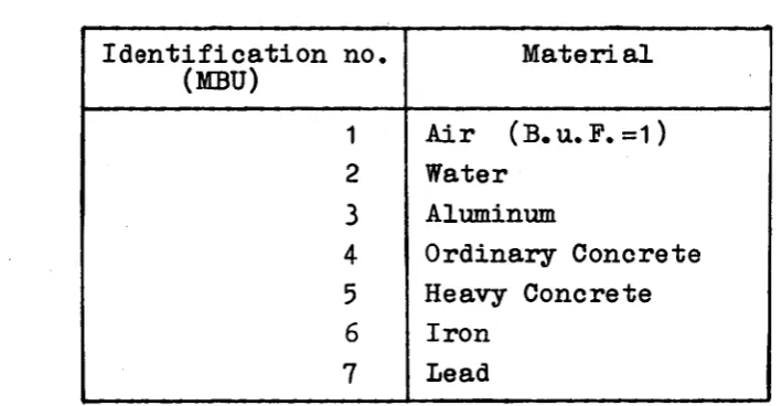
c) data for the build-up factors (see section 3.4): for

each of the 7 materials of Table 6, and each of the 7

gamma groups, we need:

Β(ΐ

), t

= i . 5 , i =0 to 6; table of B. u. P. vs. dista­

nce in m. f. p.

oi(m· ) andy5(m') coefficients which take into account

the transition from material m' to the material

considered; m'=1 to 7.

All the data l i s t e d have been written on the library t a ­

pe, behind the neutron data library.

Table 6

List of materials for which the Build-up-Factors have

been calculated.

Identification

(MBU)

no.

1

2

3

4

5

6

7

Material

Air (B.u. P. =1)

Water

Aluminum

Ordinary Concrete

Heavy Concrete

42

-4. USER'S MANUAL

4. 1 Computer Requirements

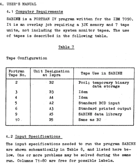
SABINE is a FORTRAN IV program written for the IBM 7090. It is an overlay job requiring a 32K memory and 7 tape units, not including the system monitor tapes. The use of tapes is described in the following table.

Table 7

Tape Configuration

Port ran Tape No.

2

3

4

5

6

9

10 .

Unit Designation at Ispra

B2

B3 A4 A2 A3 A5 B5

Tape Use in SABINE

Pool; temporary binary data storage Idem

Idem

Standard BCD input

Standard printed output SABINE data library Same as B2

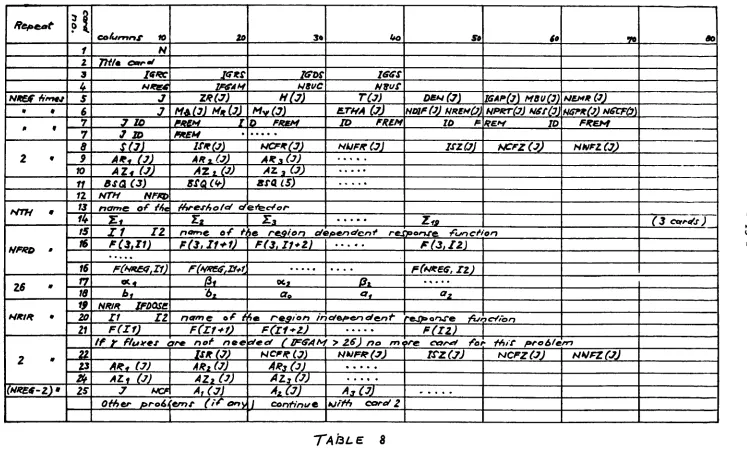
4.2 Input Specifications

Repeat

NREjf Arno*

* ·

* f

2 ·

Nm »

NFRD »

16 »

HRIR · 2 (URES-Ζ)ι

lì

n

4

CO fu m rt S 10

N 7tH· o*r*

19RC H*m*

J 3

7 ID j m S (3) A*< (3) A2<(3j BSQ (3) HTM NFZÙ name of ¿6c

Σ «

11 Σ Ζ PC3.I1)

FC«X£.<t,Il) Ä 1

6 ,

NR/R IFÛQSE ΣΙ ΣΖ

FUfJ

20

l<s*s

IFffAM

Z*(7) MA (J] HnOl

F*t* t

FREM ISR(j) AHi(j)

AT

t φ

ESQ. fr)

3 ·

IffOS H8UC

HÎ7) M* (3)

D FRMM

NCFR(7) AR 3 O)

AZ 3 U)

ssa LS)

thresh o lef </e»fec■^'e>/,·

Σ* Σ3

i*o

IGCS Ν*υΓ T(7) BTr/A (7)

ID FREM

Ν kJ FR (7)

m a * · ·

Se

DEH (7) NOlFfJj Ν'REH (3)

10 F

ISZC7J

ZÍJ,

to

IGAP(j) M8U(J)

70

MEM* (¿J

NPRT(J) H6tCÕi N6TR(J) »¿"CFC}) R£»f ID

NCFZ(JJ

name of the region cfèpen&cnf response function

F (3,11+1)

rfw&jjjr+i

ßl Ò,

name or" h F(Zf+0

F(3, ΣΙ*Ζ)

• · · · « oc.

α9

4 « region in

• · · · Ä

« ,

ìofepenofent

Ρ (3,1 Ζ)

FCNREG, ΣΖ) Οζ

rejponxe -fatnctiOn

F(Z1+Z) Í F (ΣΖ)

FREM

NHFZ (3)

If ÌT fluyes are not neeoteef ( FGAM > Z6) no more cor** rar fhit proàtèm

A*4 (3) AL, (J)

7 HCft

IS It (7) A*t (J)

AZi (3)

A,(7J

Other proé/Çemf (ff ony,

1

NCFR (J) A*3 (JJ

AL, (3)

Λ* (7)

I contìnue

NUFR(7j

A,C3J

Klt'fh cord 2

IS-ZC7) r4CFZ(7) rJVFZCTj

40

(3 Cern/s)

00

- 44

Card Columns Format Name D e s c r i p t i o n

1 2 1-10 2-70 1-10 110 N 14A5 110 IGRC

11-20 110 IGRS

21-30

31-40

110 IGDS

n o iGss

1-10

11-20

110 NREG

110 IFGAM

Number of problems t o be s o l v e d T i t l e c a r d ; t h e c o n t e n t of t h i s c a r d i s p r i n t e d a s h e a d - l i n e i n each page of t h e o u t p u t .

Index f o r t h e c o r e geometry ( s e c t i o n 1.2)

0 for plane geometry

1 for cylindrical geometry

2 for spherical geometry

3 for disk geometry

Index of the shield geometry, for

the calculation of removal neutrons

and gamma radiation from the core.

0 for plane slabs

1 for cylindrical shells

2 for spherical shells

Index of the shield geometry for

the solution of the diffusion

equa ti on.

Same possibilities as IGRS.

Index of the shield geometry for

the calculation of the ( secondary)

gamma flux originated inside the

shield

0 infinite plane slabs

1 cylindrical shells

2 spherical shells

3 disks

Number of regions ^22 (2 source

regions and no more than 20

shielding regions)

Controls the calculation of the

f

amma sources: if IFGAM>26

number of neutron groups) no

gamma calculation is performed.

When IFGAM < 26 the gamma sources

are calculated considering

be-sides the fission source, the

reactions (n, # ) and (n,n'jf ) with

neutrons of the groups I

>

IFGAM.

45­

21­30 110 NBUC" 31­40 110 NBUS.

Determine the form of the Build­up­Factor for the Core

and the Shield gamma radiation respectively (section 3.4)

One card 5 is needed for each region J, J=1, NREG. 5 1­10 110 J Index 6f the region

11­20 F10.0 ZR(J) Thickness of the region (cm) 21­30 F1Q.0 H(J) For plane geometry not used

For cylind. geometry: height for finite cyl., zero for infinite cyl.

For sph. geometry not used

For disk geometry diameter of the disk.

31­40 F10.0 T(J) Temperature of t h e r e g i o n ( ° 0 ) 41­50 F10.0 DIN(J) Densi t y ( gr/cm3 )

51­55 15 IGAP(J) = 1 normal r e g i o n

2 t h i s r e g i o n i s an a i r gap to be t r e a t e d i n P1 approx.

( s e c t i o n 2 . 8 . 1 )

3 A i r gap witheid an/3 v a l u e s i n i n p u t ( s e c t i o n 2 . 8 . 2 )

56­60 15 MBU(J) Code number of t h e m a t e r i a l f o r the B u i l d ­ u p ­ F a c t o r of t h i s region, 61­65 15 NEMR(r) No. of elements i n t h e r e g i o n , $ 10. One c a r d 6 i s needed f o r each r e g i o n J ; t h e c o n t e n t of c o ­ lumns 41­70 need to be s p e c i f i e d only f o r s h i e l d r e g i o n s ( J > 3 ) .

J Index of the region

M9(J) Determine the fraction of the mi­

jl, /j\nimum relaxation lenght to be used R^ ' as mesh interval for the numerical M«.(J) integration alongé, R, and γ

respectively. Use Μ^=ΜτρΜγ =1 as

standard value (secxiofi 3.6) 31­40 E1O0 EEHA(J) Relative accuracy for numerical

integration (section 3.6). Use .001 as standard value.

1-10

11-15 16-20 21-25

no