A new Itinerary Planning Approach Among
Multiple Mobile Agents in Wireless Sensor
Networks (WSN) to Reduce Energy Consumption
Imene Aloui
1, Okba Kazar
1, Laid Kahloul
1, Sylvie Servigne
21LINFI laboratory, Computer science department, Biskra University, Algeria 2
LIRIS Laboratory, INSA Lyon, Lyon University, France
[email protected], [email protected], [email protected], [email protected]
Abstract: one of the important challenges in wireless sensors networks (WSN) resides in energy consumption. In order to resolve this limitation, several solutions were proposed. Recently, the exploitation of mobile agent technologies in wireless sensor networks to optimize energy consumption attracts researchers. Despite their advantage as an ambitious solution, the itineraries followed by migrating mobile agents can surcharge the network and so have an impact on energy consumption. Many researches have dealt with itinerary planning in WSNs through the use of a single agent (SIP: Single agent Itinerary Planning) or multiple mobile agents (MIP: Multiple agents Itinerary Planning). However, the use of multi-agents causes the emergence of the data load unbalancing problem among mobile agents, where the geographical distance is the unique factor motivating to plan the itinerary of the agents. The data balancing factor has an important role especially in Wireless sensor networks multimedia that owns a considerable volume of data size. It helps to optimize the tasks duration and thus optimizes the overall answer time of the network. In this paper, we provide a new MIP solution (GIGM-MIP) which is based not only on geographic information but also on the amount of data provided by each node to reduce the energy consumption of the network. The simulation experiments show that our approach is more efficient than other approaches in terms of task duration and the amount of energy consumption.
Keywords: wireless sensor networks; mobile agent; itinerary
planning; data load balancing, geographical distance, data size.
1.
Introduction
Wireless sensor networks (WSNs) represent an important technology which offers a new way for collecting data. The great power of sensor networks resides in their ease of deployment in a large geographic area and their good quality of service [20]. The WSN consists of a set of nodes capable to collect information from a monitored environment and to transmit these data toward the base station “the Sink” through the wireless medium. WSNs are often characterized by dense deployment in large-scale environments that are poor in terms of resources [1]. These kinds of networks suffer from insufficient storage capacity, processing and autonomy because they are usually powered by batteries which rarely, can be replaced. This leads to problems associated with power consumption during functioning of the network nodes [17].
To resolve these limitations, the research interest has increased in the design, development and deployment of mobile agent systems in wireless sensor networks. A mobile
agent is a special kind of software that migrates among the nodes of a network to perform a task (or tasks) autonomously and intelligently, in response to changing conditions in the network environment [7]. This agent realizes the objectives of its agent dispatcher. Mobile agents have been found to be particularly useful in facilitating efficient data fusion and dissemination in WSNs [12]. The majority of researches in this field are oriented towards the optimization of energy consumption in nodes through planning mobile agent itinerary. The itinerary followed during the migration of the mobile agent can have a significant impact on energy consumption. Finding an optimal sequence of visited sources is a difficult problem to solve (NP-hard problem) [16]. A number of studies have been done to solve the problem of itinerary planning in sensor networks through the use of a “single mobile agent” (so a Single Itinerary Planning or SIP). In [2], two heuristic algorithms are proposed: (i) Local Closest First (LCF), which seeks the next node with the shortest distance to the current node, and (ii) Global Closest First (GCF) that seeks the other closer node to the sink. In [3], the MADD algorithm (Mobile Agent based Directed Diffusion) is proposed. MADD is similar to LCF, but it differs in the choice of the first source node. MADD selects the farthest source node from the sink as the first source. Another study, in [4], proposed a genetic algorithm for itinerary planning of the mobile agent in the sensor networks. The genetic algorithm reduces the search space by assuming that each node cannot be visited repeatedly.
The single mobile agent based approaches (SIP: single itinerary planning) suffer from delay problem when the networks is very large and thus many source nodes have to be visited by a single agent. Another important risk, in case of SIP, is the possibility of losing the mobile agent during its migration through several sources nodes [14]. To solve these problems, related to SIP, [6, 8-11] proposed the use of “multiple mobile agents” instead of a single agent, which requires an itinerary planning for multiple agents (so a Multiple Itinerary Planning, or MIP). Itinerary planning for multiple mobile agents in WSNs, should consider the following three questions in relation to SIP [5]:
• Q1: What is the best way to defining the necessary number of mobile agents (MAs)?
• Q3: What is the best way to defining the optimal itinerary of each Mobile Agent?
In the exciting studies on MIP [6, 8-11, 14, 18-19], which will be presented at the following section, the itinerary planning is based only on geographic information. Consequently, the groups of source nodes are irregularly distributed which provide a variation in the data size among groups. Therefore, it leads to an unbalanced data among agents. The data balancing factor allows flexible control over the compromise between energy cost and the task duration [8]. We observed that the data size has a direct impact on the energy consumption as well as on data collection task duration. When the agent collects an increasing amount of data in its memory, the agent size will increase accordingly, and so it will take more time and consume more energy to return to the Sink. So the balance among mobile agents at the level of data size optimizes the data collection task duration over the network and also decreases the percentage of data loss.
For these reasons, our study takes charge of resolving this problem, where we are materialized to find the optimal itinerary among multiple mobile agents in WSN in relation with the data size provided by each source node and the distance between them. Our study provides a new way for determining the number of mobile agents and for grouping source-nodes.
This paper is organized as follows. In the second section, we present some previous work related to the problem of MIP (Multiple mobile agent Itineraries Planning). In the third section, we explain the principle of our approach and how to realize the data load balancing. The fourth section will explain the process of our approach, and then we will highlight our strategy through two case studies in the fifth section. Finally, the sixth section concludes this paper and proposes some suggestions for future research.
When you submit your paper print it in two-column format, including figures and tables. In addition, designate one author as the “corresponding author”. This is the author to whom proofs of the paper will be sent. Proofs are sent to the corresponding author only.
2.
State of the art on proposed MIP solutions
A number of studies have been conducted for multiple mobile agent itineraries planning in the sensor network domain. In this section, we review some of these approaches. In [6] the Centre Location-based Multi agents Itinerary Planning (CL-MIP) algorithm is proposed; the main idea is to consider the solution of multi agent itineraries planning (MIP) as an iterative version of the solution -developed for- the single mobile agent itinerary planning (SIP). In CL-MIP, the visiting area of a Mobile Agent is determined by the circle centered at a visiting central location point (VCL). Then, the source nodes within the circular area will be assigned to the mobile agent. The CL-MIP use one of SIP algorithms proposed above [2-4], for determine the path of each mobile agent. In this approach the efficiency of source grouping by a circle is not a generic solution because nodes are irregularly distributed. In addition, the radius of the
source-node’s group will also strongly affect the performance of CL-MIP algorithm, the optimal value is not measured or analysed explicitly [5].
In [19] we have the proposal Angle Gap-based MIP (AG-MIP), this proposal provides a new view of source nodes grouping that do not use the circle shape. In AG-MIP the nodes within a particular angle gap threshold θ around one central location (VCL) must be included in the same group. The main idea of AG-MIP is to connect the sink and all source nodes with beelines and the angle gaps Δθ between beelines become a critical factor to describe the relevant degree among the source nodes. The importance of AG-MIP is their way of grouping; it uses angle gap to divide the network into sectors, which lead to a contention and interferences potentially reduced among mobile agent, but the open interrogation in this approach is how to find an optimal angle gap threshold.
In [8], a Genetic Algorithm for Multi agents Itinerary Planning (GA-MIP) is proposed. To realize the GA-MIP algorithm, the idea depends to encode the “Source Node Sequence” and the “Source Node Group” into numbers as genes in the genetic evolution with randomly selection. After a number of evolution iterations, the solution corresponding to an efficient strategy of itinerary planning will be obtained. Although, extensive simulations were performed to show the performance of the GA-PMI in terms of time and energy consumption, but the complexity of higher GA-PMI calculation makes the implementation of GA-MIP still debatable [15].
The proposal in [9] considers models of MIP problems as a Totally Connected Graph (TCG). In the TCG, the vertices are the nodes of the sensor network, and the weight of an edge is estimated from the jump between the two end-nodes of the edge. The authors indicate that all source-nodes in a particular sub-tree should be considered as a group.
The authors in [10] proposed the Near-Optimal Itinerary Design algorithm (NOID). The objective of this algorithm is to find the number of mobile agents that minimize the overall data fusion cost. In NOID the geographical distance is the crucial factor to group the source nodes. It uses a compromise function to effectively include nodes that are far from the center. Build path is achieved by the adoption the constraint minimum spanning tree problem. NOID surpasses CFL and GCF, but it suffers from low working speed and high computational complexity.
the problem of WSN size increase, where more branches will be created, which will degrade the performance significantly because of the interference.
The Tree-Based Design Directions is illustrated (TBID) in [18], it is a heuristic algorithm that improves the one proposed in [10]. TBID determines the appropriate number of Mobile agents to minimize the total aggregation cost as well as it builds low cost itineraries for all agents. This algorithm also uses a greedy approach as always select the nearest node to form the binary tree. It generates low itineraries for AM, but the energy consumption is doubled in the reverse roads and interference among the huge amounts of branches.
3.
Proposed approach
Through this section, we will explain the principle of our proposal to achieve “Itinerary planning for data load balancing among multiple mobile agents in WSN”, in relation with the data size provided by each source node and the distance between them. This Principe will improve the energy preservation and reduce the task duration in WSNs. Our proposed approach can be categorized as static planning where the agent itinerary is totally determined by the sink node before the agent is dispatched. It involves the following three necessary phases to achieve planning:
• Partitioning the network based on geographical information; this phase will produce a set of partitions. Each partition can receive several mobile agents; • Determining the necessary number of mobile agents and
defining the groups of nodes to be associated for each mobile agent according to the data size provided;
• Determining the itinerary that pass throughout the source nodes grouping of each mobile agent.
The figure below depicts graphically an example of a partitioned network and the inside communication of our proposal.
Figure 1.Partitioning of the network and the inside communications
In the following paragraphs, we present the three phases of the proposed strategy with more details.
3.1 Network Partitioning
Based on geographic information, this phase is responsible for the partitioning of the network. This partitioning is made according to the distance between the sensor node (Nearest
grouped together) to guarantee the shortest paths among nodes in the same partition. Our strategy depends for partitioning the network into k clusters through the “k-means” algorithm [13]. It is an efficient easy method in time and memory. It can be used with large databases (thousands of sensors). K-means technique is a widely adopted in WSN for load the clustering task. The clustering is a critical task in Wireless Sensor Networks for energy efficiency and network stability [21]. It due to partition the nodes into groups called clusters. In each cluster, a node is chosen to be the cluster head. This cluster head accountable to collect data messages from the nodes belonging to its cluster [22]. In this paper, the mobile agents are responsible to collect a data from the network. And for spread work areas between agents, we adopted the k-means algorithm to make this task.
The k-means algorithm aims at partitioning the n sensor nodes Si: i∈ [1,2, …,n] into k partitions Pj ∈ [1,2, …,k]
(k ≤ n) from k centers “Cj” chosen arbitrarily. This algorithm
aims at minimizing the distance among the sensors nodes “Si” within each partition “Pj”:
∑ ∑
= =
−
k
j n
i
j i p
C S
1 1
2
min
arg (1)
Where Si−Cj 2 is a distance measure among a sensor nodes “Si” and the partition centre “Cj”.
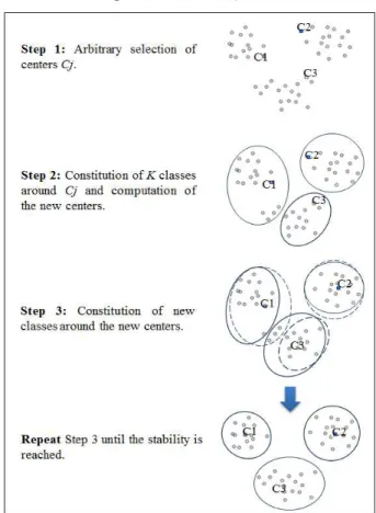
Figure 2.Network partitioning using the k-means method
The method computes the distance among all sensor node Si
and all the initial centers “Cj” and affects each sensor node to
the nearest partitions “Pj”. Once all the sensor are affected,
partition “Pj” and denotes this centers as the new centers
“Cj”. This process is repeated until the partitioning reaches
some stability (Indeed, a threshold can be fixed as a stop condition).
∑
== n
i i S
j P j G
1
1 (2)
The Figure 2 shows graphically the evolution of partitioning using k-means method:
Once the partitioning is done, we select in each cluster a particular node as a “partition-leader”; it is the nearest node to the gravity center of the partition. This node (leader) will be responsible for sending the size of all the detected data by all the nodes inside its partition, to the sink. In our task, the data size plays an important role in determining the number of mobile agents and the list of sources nodes associated to each agent.
3.2 Determine the mobile agents number and their associated groups of source nodes
After partitioning the network, the number of mobile agents required for the aggregation of data and the groups of source nodes associated for each agent are determined simultaneously for each partition. We propose a strategy that we call “GIGM” (the Greatest Information in the Greater Memory) to make this task.
The idea of our proposition consists of a set of sensor nodes
Si: i ∈ [1, n]: (n ∈ N*), included in k partition Pj: j ∈ [1, k]
where (k ≤ n), as presented above. Also, there are “m” source nodes in the network, denoted by S’h: h ∈ [1, m], where
S’⊂S, and we have RDS[h] the raw data size provided by
each source nodes h. This RDS allow us to determine the number of mobile agents deployed in each partition.
In our proposed, the number of agents varies from one partition to another, depending on the data size provided by each source nodes inside their partitions and the free memory size of mobile agent. So we seek the number which is able to collect all the data of the network.
To determine the number of mobile agents, we start with an initial number “NbMA”, where “NbMA” is computed using the
the equation (3):
MMA j DS NbMA ≈ ( ) (3) Such that:
DS(j): the size of the sensed data in the partition ‘j’ composed of y source nodes. This size is computed using the following equation:
[ ]
∑
=
≈
y
x
x RDS j
DS
1
)
( (4)
Where
RDS: the raw data size provided by each source nodes y.
And
MMA: the free memory size of mobile agent (initially the
same memory size for all the agents).
This initial number "NbMA" of mobile agents can be increased
over the execution of “GIGM Algorithm” until the sufficient number of agents (necessary number to collect all the data in each partition of the network) is obtained.
In order to determine VG(MAx) : x ∈ [1, a] the groups of
source nodes that must be visited by each mobile agent MAx,
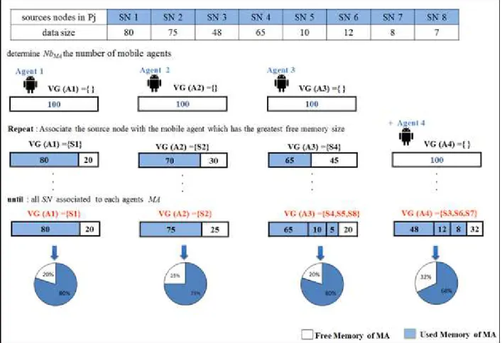
the strategy GIGM is based on the following principle: “The Greatest quantity of Information is associated with the mobile agent who has the Greater free Memory size”. This strategy ensures the load data balancing among mobile agents.
Below, we present he algorithm of the GIGM strategy and the Figure 3 shows its execution.
Pseudo code implementation of GIGM algorithm:
Data:
S’: set of source nodes
VG(MAx) ←∅ : source nodes groups
RDS[h]: raw data size provided by each source nodes h. MMA: memory size of a mobile agent
BEGIN
For all partitions Pj
o Calculate the initial number of mobile agents :
MMA j DS
NbMA
) ( ≈
Repeat
o Find the source node which has max(RDS[h]);
o associate this node with the mobile agent which has the greatest free memory size (max(MMA[x]));
VG(MAx) ← { h ∈ S’ | max ( RDS[h] ) } o Update the free memory size of this agent:
MMA[x]= MMA[x]-RDS[h];
If all MMA[x]< RDS[h] (all the free memories in all mobile agents are not sufficient to contain this information) then Update the number of agent: NbMA =NbMA+1
Until (all source nodes are associated to mobile agents); End for
Figure 3.The GIGM strategy execution (a demonstrative example).
3.3 Itinerary planning for each mobile agent
After determining the number of mobile agents with its corresponding group of source nodes, the itinerary that pass throughout this source nodes, should be determined for each mobile agent. In our study aims requires the uses of LCF (Local Closest First) algorithm [2], to determine the itinerary of each agent when visiting its nodes. This algorithm finds an optimal way avoiding redundancies. It seeks the next node with the shortest distance to the current node where the Sink is the starting and the ending point for the itinerary.
4.
Simulation and performance evaluation
4.1 Simulation
In order to compare the performance of GIGM-MIP solution with CL-MIP and GA-MIP, we carry out simulations in MATLAB7.1. Following the most popular network model in MA research, the nodes are uniformly deployed within a 1000m×500m field, and the sink node is located at the centre of the field and multiple source nodes are randomly distributed in the network. To verify the scaling property of our algorithms, we select a large-scale network with 800 nodes. The parameters necessary for the network, MA and GA-MIP are shown in following Table I.
Table 1.Basic simulation parameters
PARAMETERS FOR NETWORK
Network size 1000 m x500m
Node Distribution Random Radio Transmission
Range 60 m
Number of Sensor Nodes 800
Raw Data Size 2048 bits
PARAMETERS FOR MOBILE AGENTS SYSTEM
Raw Data Reduction
Ratio 0.8
Aggregation Ratio 0.9 MA Code Size 1024 1024 bits MA Accessing Delay 10 10 ms Data Processing Rate 50 Mbps PARAMETERS FOR GA-MIP GA Iteration Times 1500 GA Search Spaces 300 Sequence Crossover
Ratio 0.9
Figure 4.Visualization of GIGM-MIP with 5 MAs
The Fig.4 shows the visualization of the GIGM-MIP strategy, in which five mobile agents are sent by the sink node to aggregate the data in 80 source nodes simultaneously. 4.2 Performance evaluation
In order to evaluate the performance of GIGM-MIP, from the simulation results that are made in the previously defined environment "MATLAB 7.1", we consider the following three performance metrics:
a)Data load balancing among multiple mobile agents
The irregular distribution of sensor nodes in WSN provides a variation in the data size among clusters. Therefore, it leads to an unbalanced distribution of data among agents. When the agent collects an increasing amount of data in its memory, the agent size will increase accordingly, and so it will take more time and consume more energy to return to the Sink. So a balance distribution of data size among mobile agents has influences significantly on the task duration and the energy consumption.
To determine the effectiveness of the GIGM-MIP strategy on the level of data load balancing among mobile agents, Figs.5 is provided in this subsection.
Figure 5.The data load balancing result among 5 MAs in the GIGM-MIP, CL-MIP and GA-MIP.
The simulations result in Fig.5 shows that the GIGM-MIP strategy allows a balancing distribution of the data on the set of agents. The percentages of data collected by each one of the five agents are distributed between 35% and 30%. Thus,
GIGM-MIP allows agents to collect a data size almost equivalent. This proves that this strategy achieves a data load balancing among agent both CL-MIP and GA-MIP could not achieve.
b)Task Duration
In this sub-section, we show the simulation result of the impact of number of source nodes on task duration. In an MIP algorithm, since multiple agents work in parallel, the task duration is the delay of the agent which returns to the sink at last.
Figure 6.The impact of number of source nodes on Task Duration.
As shown in Fig.6, GIGM-MIP algorithm has large advantage in terms of task duration, which is convergent with GA-MIP and spaced with CL-MIP that cost a longer task duration. The reason behind performance of GIGM-MIP is the determination of the sets of source-nodes based on geographic information and a data size detected to achieve load data balancing among MAs.
c)Energy Cost
In the following Figure, we show the simulation result of the impact of number of source nodes on energy cost.
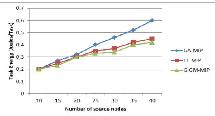
Figure 7.The impact of number of source nodes on Energy Cost.
In Fig.7, the energy consumption of GA-MIP algorithm is a higher than that of CL-MIP and GIGM-MIP algorithms. This is due to its higher complexity of calculation. As regards the energy consumption of GIGM-MIP is approximately equal to the CL-MIP result. The latter both algorithms use the same algorithm for determine the path of each mobile agent (CLF algorithm), which is due a low complexity of calculation. MA 2 itinerary
MA 3 itinerary MA 4 itinerary MA 5 itinerary Sink node
5.
Conclusion
The multiple MAs approach enhances the capacity of WSNs. It has a positive factor in terms of energy consumption. However, the exciting MIP approaches are based only on geographic information; consequently, it causes the emergence of the problem of unbalancing of data among mobile agents. In this work, we have presented a new method for finding the optimal itinerary for load data balancing among multiple mobile agents in WSN. Our study provides a new way to determine the number of mobile agents with its source-nodes grouping. The proposed strategy GIGM-MIP is based on the balance between geographic information and data size. This principle of GIGM-MIP has a specifically positive impact in terms of the task duration and the amount of energy consumed.
The next step of this work is to evaluate the performance of GIGM-MIP in a Wireless Multimedia Sensor Networks (WMSN) which has high data size.
References
[1] N. Meghanathan, “Grid Block Energy Based Data Gathering Algorithms for Wireless Sensor Networks”, International Journal of Communication Networks and Information Security (IJCNIS), Vol. 2, No. 3, 2010.
[2] M. Chen, S. Gonzalez, & V.C. Leung, “Applications and design issues for mobile agents in wireless sensor networks”, IEEE Wireless Communications, vol. 14, No. 6, pp. 20–26, 2007.
[3] M. Chen, T. Kwon, Y. Yuan, Y. Choi, and V. Leung, “MADD. Mobile agent-based directed diffusion in wireless sensor networks”, EURASIP Journal on Applied Signal Processing, vol. 2007, No. 1, pp. 219–219, 2007.
[4] Q. Wu, N.S.V. Rao, J. Barhen, & al, “On computing mobile agent routes for data fusion in distributed sensor networks”, IEEE Transactions on Knowledge and Data Engineering, Vol. 16, No. 6, pp. 740–753, 2004.
[5] X. Wang, M. Chen, T. Kwon, & H.C. Chao, “Multiple mobile agents’ itinerary planning in wireless sensor networks: survey and evaluation”, IET Commun, Vol. 5, No. 12, pp. 1769– 1776, 2011.
[6] M.Chen, S. Gonzlez, Y. Zhang, & V.C. Leung, “Multi-agent itinerary planning for sensor networks”, Conf. Heterogeneous Networking for Quality, Reliability Security and Robustness, Las Palmas de Gran Canaria, Spain,2009.
[7] M. Chen, “Itinerary Planning for Energy-Efficient Agent Communications in Wireless Sensor Networks”, IEEE Transactions on Vehicular Technology, Vol. 60, No. 12, pp. 3290-3299, 2011 .
[8] W. Cai, M. Chen, T. Hara, L. Shu, “GA-MIP: genetic algorithm based multiple mobile agents itinerary planning in wireless sensor network”, Proc. Fifth Int. Wireless Internet Conf (WICON), pp. 1-8, Singapore, 2010.
[9] M. Chen, W. Cai, S. Gonzalez, & V.C. Leung, “Balanced itinerary planning for multiple mobile agents in wireless sensor networks”, Proc. Second Int. Conf. Ad Hoc Networks (ADHOCNETS 2010), Victoria, Canada, 2010.
[10]D. Gavalas, A. Mpitziopoulos, G. Pantziou, & C. Konstantopoulos, “An approach for near-optimal distributed data fusion in wireless sensor networks”, Springer Wireless Networks, Vol. 16, No. 5, pp. 1407–1425, 2009.
[11]D. Gavalas, G. Pantziou, & C. Konstantopoulos, “New Techniques for Incremental Data Fusion in Distributed Sensor Networks”, In Proceedings of the 11th Panhellenic Conference on Informatics (PCI’2007), pp. 599–608, 2007.
[12]H. Qi, F.Wang, “Optimal itinerary analysis for mobile agents in Ad Hoc wireless sensor networks”, Proc. IEEE 2001 Int. Conf. Communications (ICC 2001), Helsinki, Finland, 2001. [13]J.P. Nakache, J. Confais, “Approche pragmatique de la
classification: arbres hiérarchiques, partitionnements”, Edition TECHNIP, Paris, 2005.
[14]A. Mpitziopoulos, D. Gavalas, C. Konstantopoulos, G. Pantziou, “CBID: a scalable method for distributed data aggregation in WSNs”, Hindawi Int. J. Distrib. Sens. Netw, Vol. 2010, 2010.
[15]A.N. Rani, L. Dole, “GA based optimal itinerary planning for multiple mobile agents in wireless sensor networks”, International Journal of Innovative Research in Computer and Communication Engineering, Vol. 1, No 2, 2013.
[16]Y. Xu, & H. Qi, “Mobile Agent Migration Modeling and Design for Target Tracking in Wireless Sensor Networks”, Ad Hoc Networks, vol. 6, No. 1, pp. 1–16, 2008.
[17]A. Sardouk, L. Merghem-Boulahia, & D. Gaïti, “Agent-Cooperation Based Communication Architecture for Wireless Sensor Networks”, The 1st IFIP wireless days conference, pp. 1-5, 2008.
[18]C. Konstantopoulos, A. Mpitziopoulos, D. Gavalas, G. Pantziou, “Effective determination of mobile agent itineraries for data aggregation on sensor networks”, IEEE Trans. Knowl. Data Eng, vol. 22, No. 12, pp. 1679–1693, 2010. [19]M. Chen, S. Gonzalez, V. Leung, “Directional source grouping
for multi-agent itinerary planning in wireless sensor networks”, Proc. Int. Conf. ICT Convergence (ICTC), Jeju Isaland, Korea, pp. 207-212,2010.
[20] M. Dong, K. Ota, M. Lin, Z. Tang, S. Du, H. Zhu, “UAV-assisted data gathering in wireless sensor networks”, Springer of Supercomputing, vol. 70, No. 3, pp. 1142–1155, 2014. [21]W. Gicheol and C. Gihwan, “Securing Cluster Formation and
Cluster Head Elections in Wireless Sensor Networks”, International Journal of Communication Networks and Information Security (IJCNIS), Vol. 6, No. 1, 2014.