arXiv:1605.00289v1 [astro-ph.SR] 1 May 2016
MULTIPLE GAPS WITH LARGE GRAIN DEFICIT IN THE PROTOPLANETARY DISK
AROUND TW HYA
Takashi Tsukagoshi1, Hideko Nomura2, Takayuki Muto3, Ryohei Kawabe4, Daiki Ishimoto2,5,
Kazuhiro D. Kanagawa6, Satoshi Okuzumi2, Shigeru Ida7, Catherine Walsh8, Tom J. Millar9
1College of Science, Ibaraki University, Bunkyo 2-1-1, Mito, Ibaraki, 310-8512, Japan;
2Department of Earth and Planetary Sciences, Tokyo Institute of Technology, 2-12-1 Ookayama, Meguro, Tokyo,
152-8551, Japan
3Division of Liberal Arts, Kogakuin University, 1-24-2 Nishi-Shinjuku, Shinjuku-ku, Tokyo, 163-8677, Japan
4National Astronomical Observatory of Japan, 2-21-1 Osawa, Mitaka, Tokyo 181-8588, Japan
5Department of Astronomy, Graduate School of Science, Kyoto University, Kitashirakawa-Oiwake-cho, Sakyo, Kyoto,
606-8502, Japan
6Institute of Physics and CASA∗, Faculty of Mathematics and Physics, University of Szczecin, Wielkopolska 15, 70-451
Szczecin, Poland
7Earth-Life Science Institute, Tokyo Institute of Technology, 2-12-1 Ookayama, Meguro, Tokyo 152-8550, Japan
8Leiden Observatory, Leiden University, P. O. Box 9513, 2300 RA Leiden, The Netherlands
9Astrophysics Research Centre, School of Mathematics and Physics, Queen’s University Belfast, University Road,
Belfast BT7 1NN, UK
ABSTRACT
TW Hya at 138 and 230 GHz with the Atacama Large Millimeter/Submillimeter Array.
Our observations revealed two deep gaps (∼25–50 %) at 22 and 37 au and shallower
gaps (a few %) at 6, 28, and 44 au, as recently reported by Andrews et al.(2016). The
central hole with a radius of∼3 au was also marginally resolved. The most remarkable
finding is that the power-law index of the dust opacity β, derived from the spectral
index α between bands 4 and 6, peaks at the 22 au gap with β ∼ 1.7 and decreases
toward the disk center to β ∼ 0. Our model fitting suggests that the overall disk
structure can be reproduced with the inner hole and the gaps at 22 and 37 au. The
most prominent gap at 22 au could be caused by the gravitational interaction between
the disk and an unseen planet with a mass of .1.5 MNeptune although other origins
may be possible. The planet-induced gap is supported by the fact that β is enhanced
at the 22 au gap, indicating a deficit of ∼mm-sized grains within the gap due to dust
filtration by a planet. Alternatively, the destruction of large dust aggregates due to the
sintering of major volatiles might cause the multiple ring structure. We also find weak
sinusoidal patterns with wavelengths of 5–10 au, which may be related to dynamical
instabilities within the disk.
Keywords: protoplanetary disks — stars: individual(TW Hya)
1. INTRODUCTION
Protoplanetary disks are the birthplaces of planets. The complex structures of protoplanetary
disks such as spiral arms, inner holes, and gap and ring, recently reported by high-resolution infrared
observations (Akiyama et al. 2015; Muto et al. 2012; Tsukagoshi et al. 2014), are believed to be
potential evidence of unseen planets in the disk. Most recently, high-resolution observations with
Partnership et al. 2015). Since submillimeter emission better traces the midplane density structures
than infrared, the gaps and rings are thought to be direct evidence of the absence and enhancement
of disk material, and therefore related to the planet formation process. The origin of multiple gaps
and rings is still under debate: several theoretical studies predict a formation scenario due to material
clearance by planets (Tamayo et al. 2015;Kanagawa et al. 2015), replenishment of small dust grains
by sintering of molecules (Okuzumi et al. 2016), or secular gravitational instability (Takahashi &
Inutsuka 2014).
TW Hya is a 0.8M⊙ T Tauri star surrounded by a disk at a distance of ∼54 pc (e.g., Andrews et
al. 2012). Since the disk is almost face-on with an inclination angle of 7◦ (Qi et al. 2004), TW Hya is
one of the best astronomical laboratories to investigate the radial structure of protoplanetary disks.
The disk mass has been measured to be>0.05M⊙ from HD line observations by theHerschelSpace
Observatory, indicating that it is massive enough to form a planetary system (Bergin et al. 2013).
Recently, a gap in the dust emission has been found at 20–30 au by submillimeter and near infrared
observations (Akiyama et al. 2015; Nomura et al. 2016), which is possibly associated with the CO
snow line (Qi et al. 2013). Most recently, Andrews et al. (2016) reported the existence of multiple,
axisymmetric annuli at 22, 37, and 43 au at a spatial resolution of ∼1 au. The depth and width
of the submillimeter gap at 20–30 au is consistent with clearing by a super-Neptune mass planet
(Nomura et al. 2016). However, no clear consensus has been reached yet on the origin of the gap due
to the lack of corresponding information on the dust size distribution with the comparable spatial
resolution. In this paper, we report multi-frequency observations of the disk around TW Hya with
ALMA to probe the detailed disk structure and the change of dust spectral index across the dust
gaps and rings at a spatial resolution of ∼3 au.
High-resolution continuum observations at bands 4 and 6 (138 and 230 GHz) with the ALMA were
carried out on 2015 December 1 and 2 (2015.A.00005.S). In the observation period, 36 of the 12-m
antennas were operational and the antenna configuration was in transition from C36-7 to C36-1,
resulting in maximum baselines of 6.5 and 10.4 km for band 4 and 6, respectively. We employed the
Time Division Mode of the correlator, which is optimized for continuum observations. The correlator
was configured to detect dual polarizations in 4 spectral windows with a bandwidth of 1.875 GHz
each, resulting in a total bandwidth of 7.5 GHz for each observed band. The amplitude and phase
were calibrated by observations of a quasar J1103-3251, and J1037-2934 was used for absolute flux
calibration. The observed passbands were calibrated by 5 min observations of J1037-2934 and
J1107-4449 for band 4 and 6, respectively.
The visibility data were reduced and calibrated using the Common Astronomical Software
Appli-cation (CASA) package, version 4.5.0. After flagging bad data and applying the calibrations for
bandpass, complex gain, and flux scaling, the corrected visibilities were imaged by the CLEAN
al-gorithm. The visibilities at band 6 with uv lengths >3000 kλwere flagged out because of significant
phase noise. The uv sampling for baseline .200 kλ was particularly sparse along the north-south
direction (i.e., v axis of the uv coverage) for both bands 4 and 6 data. This causes artificial structure
in the resultant image due to false reconstruction by the CLEAN deconvolution method. We have
downloaded band 6 archival data (2012.1.00422.S; PI: K. ¨Oberg), in which the maximum baseline
is 650 m (∼500 kλ), these data were combined with our band 6 data after fixing the phase center.
There were no available short-baseline data at band 4, hence only the long-baseline data were used
for imaging. The obtained band 4 image appears similar to that with the band 6 image, however,
there is slight asymmetry in the intensity distribution at band 4. To improve the image fidelity, we
performed the iterative self-calibration imaging for each band data using the initial CLEAN image
Using all of the corrected visibilities after the iterative self-calibration imaging, we constructed
a combined image of the band 4 and 6 (190 GHz) data with the multi-frequency synthesis (MFS)
method and taking into account the spectral index (nterm=2in CASACLEANtask). Briggs
weight-ing with robust=0.0 was employed for the deconvolution, and we also employed the multiscale option
with scale parameters of 0, 5, and 15 for better reconstruction of extended emission. The achieved
spatial resolution of the combined image is 72.7×47.8 mas, with a position angle of 52◦.9,
correspond-ing to 3.9×2.9 au. The noise level is 15.7 µJy beam−1.
3. RESULTS
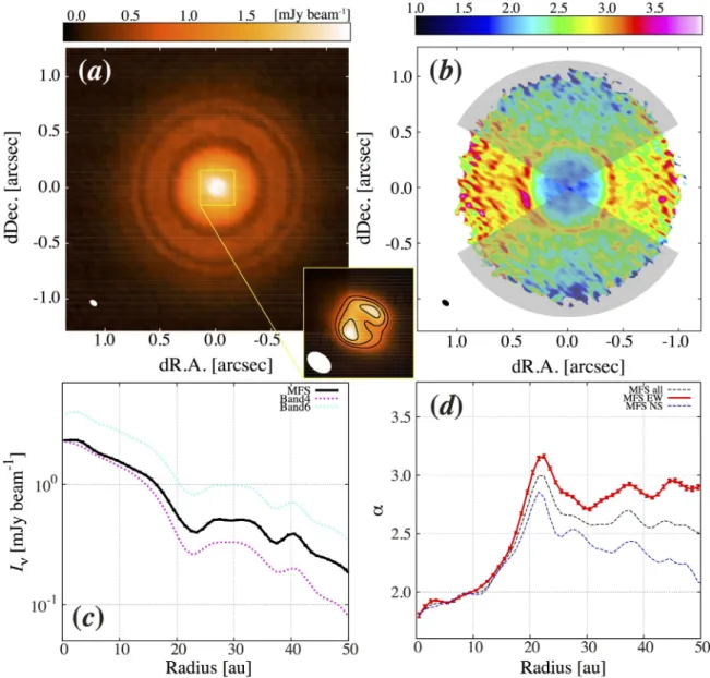
Figure1(a) shows the combined image of the band 4 and 6 data with the MFS method (hereafter
MFS image). The MFS image shows circular symmetric multiple gaps and rings. In addition, we
have resolved an inner hole with radius ∼ 3 au as predicted from analysis of the spectral energy
distribution (Calvet et al. 2002). The total flux density is 386.3±0.6 mJy at 190 GHz (SN∼ 150),
which agrees well with the previous estimation at submillimeter wavelengths (Qi et al. 2004;Andrews
et al. 2012). There is no appreciable deviation from circular symmetry in the gaps. To confirm the
gap structures, we plot the deprojected radial profile in figure 1(c). There are two prominent gaps
at 22 and 37 au, and relatively weak decrements of the surface brightness are also seen at 6, 28, and
44 au. These observed features agree with those found by recent high-resolution (∼1 au) observations
at band 7 (Andrews et al. 2016).
Figure 1(b) shows the spatial variation of the spectral index α (see eq. (2) for definition). The
obtained spectral index map is highly non-axisymmetric, and it is likely to be artificial due to the
remaining sparse uv coverage <200 kλ along the v-axis at band 4. To check the uncertainty, we plot
the deprojected radial profiles over different azimuthal angles in figure 1(d); the averaging over full
angles from −30◦ to 30◦ and from 150◦ to 210◦ (North-South direction). The derived profiles are
different, implying that the sparse uv coverage<200 kλcauses uncertainty in the value ofαespecially
at larger radii. Additional observations to gain better uv coverage at short baselines in band 4 are
required to obtain a better quality map of α. The EW direction data is the most reliable because
the sparse uv distribution appears roughly along the north-south direction and because the
intensity-weighted mean value of the spectral index agrees well with a previous measurement for the entire
disk (Pinilla et al. 2014). Hence, we use the EW direction data in all subsequent analysis, and the
shadows in figure 1(b) indicate locations where the value of α is expected to be unreliable.
The intensity Iν(R) and the spectral index α(R) are related to the dust temperature Td(R), the
optical depth τν(R), and dust opacity index β(R) by
Iν(R) =Bν(Td(R)) (1−exp [−τν]) (1)
and
α(R)≡ dlog(Iν)
dlogν = 3− T0
Td(R)
eT0/Td(R)
eT0/Td(R)−1+β(R)
τν(R)
eτν(R)−1. (2)
Here, Bν(T) is the Planck function, h is Planck’s constant, c is the speed of light and T0 = hν/kB
where kB is Boltzmann’s constant. If we assume one of Td(R), τν(R), or β(R), it is possible to
derive the other two parameters from the MFS data. Here, we assume that Td(R) is given by
Td(R) =T10(R/10 AU)−0.3 and vary T10 from 22 to 30 K. This assumption is based on the fitting of
the model result in Andrews et al. (2012), where T10 ∼ 22 K is the best fit value. We use several
different temperatures to see how temperature affects the derived physical quantities. We restrict
ourselves to T10 > 20 K because otherwise the gas temperature would fall below the brightness
temperature in the inner regions (R .10 au).
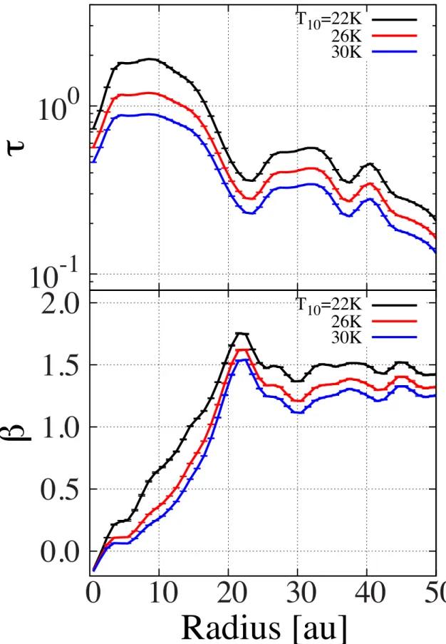
Figure 2 shows the radial profiles of the optical depth τ and the opacity index β. The disk is
contrast with HL Tau (ALMA Partnership et al. 2015;Pinte 2016), where an optically thick region
extends to much larger radii R.40 au. We see a prominent drop in the optical depth at R <5 au,
which likely corresponds to the inner hole (Calvet et al. 2002). The optical depth profiles have two
dips at R∼22 au and ∼37 au.
One of the most remarkable feature of the β profile is the peak at ∼22 au, which is exactly the
location of the gap in the surface brightness profile. This is strong evidence that small dust grains
are more abundant within the gap than at other locations in the disk. Overall, the opacity index β
increases from∼0 to ∼1.7 with radius up to∼20 au, beyond which the estimate ofβ may be affected
by the uncertainties in α discussed in the previous section. Radially increasing profiles of β are also
seen in other T Tauri disks (P´erez et al. 2012).
We note that it is possible to derive Td(R) and τ(R) by assuming β(R) or to derive β(R) and
Td(R) by assuming τ(R). To confirm that τ(R) really has a gap and/or β increases within the gap,
additional data from several different bands are necessary.
4. DISCUSSION
4.1. Structures of the Disk and Gaps
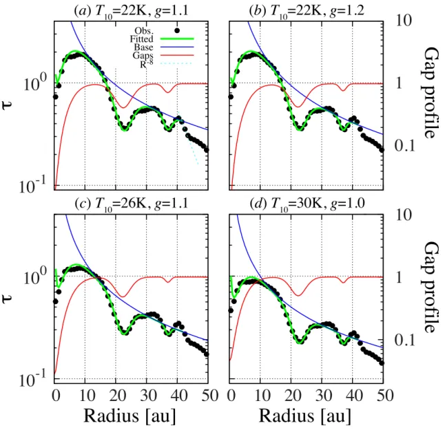
To quantify the gap width and depth, we fit the radial profiles of the optical depth τ(R) using
a model that has an inner hole and two gaps centered at ∼22 and ∼37 au. We assume that the
background profile is given by a power-law with index g, τbg =τ0(R/10 au)−g, and the shape of the
gap is assumed to be Gaussian with a depth relative to background, Ag, position rg and width, wg,
fgap= 1 + 10Ag −1
exp
−(R−rg) 2
w2 g
. (3)
We use three Gaussian functions to represent the inner hole, where rg is fixed to zero, and the two
deepest gaps at 22 and 37 au, i.e., we fit the radial profiles of τ(R) by the function
Figure 1. (a) Combined image of bands 4 and 6 with the MFS method. The ellipse at the bottom-left corner shows the synthesized beam. Inset shows a close-up view (0′′.3×0′′.3) for emphasis of the central structure.
The contour indicates 130, 140, and 150σ. (b) Spectral index map derived from the MFS method. The shadowed area indicates where the value of the spectral index is unreliable due to the inner hole of the uv coverage. (c) Radial profiles averaged over full azimuthal angle. The flux density of MFS is shown in black and those of bands 4 and 6 data are shown in magenta and cyan, respectively. The error bar shows the standard error through the azimuthal averaging. (d) Radial profiles of the spectral index α. The black line shows the profile averaged over the entire azimuth. The red and blue lines are the profile along the east-west (azimuth angle of 60–120◦ and 240–330◦) and north-south (−30–30◦ and 150–210◦) directions, respectively.
10
-1
10
0
τ
T
10
=22K
26K
30K
0.0
0.5
1.0
1.5
2.0
0
10
20
30
40
50
β
Radius [au]
T
10
=22K
26K
30K
Figure 2. Radial profile of the optical depth at 190 GHz (top) and β (bottom). The cases forT10=22, 26,
To investigate the uncertainty of the parameters, we assume several values ofg and obtain the best-fit
gap parameters by the least square method for each value ofg. The fit is restricted within R <42 au
since it is difficult to model the drop in τ(R) at larger radii (see below).
Table 3shows the best-fit parameters with different values of g and T10 and figure 3 shows several
examples: g =1.1 and 1.2 with T10 =22 K, g =1.1 with T10 =26 K, and g =1.0 with T10 =30 K.
The overall trend of the radial variation of τ(R) is well reproduced. The locations of the gaps, rg,
are well constrained for both gaps and the width of the 22 au gap is also well constrained while the
uncertainty of the width of the 37 au gap is large. The depths of the 22 au gap and 37 au gap are
determined within typical uncertainties of∼9% and∼43%, respectively. It is debatable whether the
37 au feature should be regarded as a gap but it may alternatively be interpreted as a part of radial
sinusoidal variation, rather than a single, isolated gap. In some cases where g is varied, the fit to the
37 au gap fails.
We see that the radial profile ofτ(R) drops rapidly at R&42 au, and it is difficult to fit the profile
with a single background power law. Hogerheijde et al. (2016) show that the radial surface density
distribution is well represented by a broken power-law, with the break at ∼47 au and the steep cutoff
(∝R−8) at outer radii. Our results are, at least qualitatively, in agreement with this model and also
our previous observations at band 7 (Nomura et al. 2016).
To investigate whether there are additional, weak structures other than the inner hole, 22 au gap,
and 37 au gap, we reconstructed the sub-mm image using radiative transfer calculations. We assume
the temperature profile with T10 = 22 K, and use the best-fitτ(R) profile withg = 1.1 to reconstruct
a surface density profile. We assume a dust opacity of 1.9 cm2 g−1 (Draine 2006) throughout the
disk to convert the optical depth to dust density. The dust particles are vertically distributed with
a Gaussian profile, with a dust scale height of Hd(R) = 0.6 au(R/10 au)5/4. The disk inclination is
simple model is constructed based on the parameters used in previous studies (Andrews et al. 2012)
except for the newly derived surface density profile having gaps. The main purpose of the modeling
is to reproduce the overall observed profile at R <42 au and to find small scale structures that may
be hidden behind the conspicuous multiple gap structures.
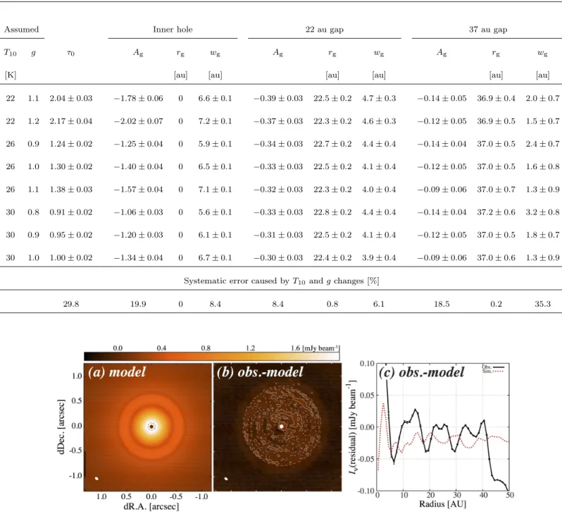
Figure 4 shows the comparison between the model and observations. The model reproduces the
observations between 5 < R < 42 au. Detailed modeling of the inner hole and outer cutoff is
necessary to reproduce the full profiles. At 5 au< R <42 au, the differences between the model and
the observations are within ∼ 5σ in the image. However, if we take the azimuthal average of the
residuals, we find a wave like radial profile, with wavelengths of 5–10 au and an amplitude of a few
%. This might indicate the presence of sinusoidal distribution of dust particles underlying the gap
profiles. To check whether the CLEAN method causes an artificial wave structure, we created the
simulated visibility of the model image using the CASAsimobservetask with appropriate parameters
and reconstructed the CLEANed image. The difference of the radial profiles between the simulated
observations and the model is also plotted in figure 4(c) and shows no significant sinusoidal pattern
like the observed data.
4.2. Origin of the Gaps and Sinusoidal Patterns
The 22 au gap parameters seem to be well constrained with a width of wg ∼4–5 au and a depth
of 10Ag ∼0.4–0.5 compared to the background τ
bg profile. In our previous studies with a spatial
resolution of ∼0′′.35 (Nomura et al. 2016), the existence of the 22 au gap is hinted at a width of 15 au
and a depth of 0.23. The mass deficit within this gap is 1.4 MJ, assuming a dust mass opacity of
1.9 cm2 g−1 at 190 GHz (Draine 2006) and a gas-to-dust mass ratio of 100, and is consistent between
the two observations.
mm-sized grain deficit inside the 22 au gap, strongly support this scenario because it is consistent with
the picture of dust filtration due to a planet (Zhu et al. 2012). Using the relationship that connects
the gap shape with the planet mass (Kanagawa et al. 2015, 2016), a planet with 1.5 MNeptune may
be responsible for the gap, assuming a viscosity parameter α = 10−3 and a disk aspect ratio of 0.05
(consistent with the assumption of T10 = 22 K). We note that similar values are derived from both
gap width and depth. This planet mass should be considered as the upper limit since the formula
by Kanagawa et al.(2015,2016) is for the gas gap and the actual dust gap may be wider and deeper
than the gas gap due to dust filtration (Zhu et al. 2012).
Alternatively, the multiple ring structure might be related to the snow lines of major volatiles
(Zhang et al. 2015; Okuzumi et al. 2016). TW Hya is suggested to have a CO snow line at ∼30 au
(Qi et al. 2013;Schwarz et al. 2016), and our observations identify a bright dust ring near this snow
line. This is consistent with the dust ring formation scenario by Okuzumi et al. (2016), in which
icy dust aggregates experience sintering, disrupt, and pileup near major snow lines. As noted by
Andrews et al. (2016), the 40 au bright ring might correspond to the snow line of N2, which has a
sublimation temperature slightly lower than that of CO.
If real, the sinusoidal distribution in dust particles may be reminiscent of dynamical instabilities
within the disk such as zonal flow patterns driven by MHD turbulence (Johansen et al. 2009),
baroclinic instability driven by dust settling (Lor´en-Aguilar and Bate 2015), and/or the secular
gravitational instability (Youdin 2011; Takahashi & Inutsuka 2014). Different dynamical processes
act under different physical conditions and therefore, better constraints on the dust disk physical
structures based on high resolution observations at other bands (e.g., Andrews et al. 2016) and
constraints of the density and temperature structures of gas component are essential in determining
Obs. Fitted Base Gaps R-8
0 10 20 30 40 50
10
-1
10
0
τ
Radius [au]
0.1
1
10
G
ap profi
le
10 10
(
c
)
T
10=26K,
g
=1.1
(
d
)
T
10=30K,
g
=1.0
0.1
1
10
G
ap profi
le
10
-1
10
0
τ
0 10 20 30 40 50
Radius [au]
Figure 3. Results of our model fitting (green) for the cases of g=1.1 and 1.2 withT10=22 K (a,b),g=1.1
withT10=26 K (c), andg=1.0 withT10=30 K (d). The black circles indicate the observed data. The blue
line indicates the fiducial (background) power-law profile. The profile of each gap is shown in red, whose axis is on the right. The dotted line in cyan in the top-left panel shows the R−8 dependence determined by
Hogerheijde et al. (2016).
This paper makes use of the following ALMA data: ADS/JAO.ALMA#2015.A.00005.S and
ADS/JAO.ALMA#2012.1.00422.S. ALMA is a partnership of ESO (representing its member states),
NSF (USA) and NINS (Japan), together with NRC (Canada), NSC and ASIAA (Taiwan), and KASI
(Republic of Korea), in cooperation with the Republic of Chile. The Joint ALMA Observatory is
Table 1. Parameters of the fitted inner hole and gaps. The error shows the standard error of the fitting. The systematic error whenT10 and gare varied is shown at the bottom row.
Assumed Inner hole 22 au gap 37 au gap
T10 g τ0 Ag rg wg Ag rg wg Ag rg wg
[K] [au] [au] [au] [au] [au] [au]
22 1.1 2.04±0.03 −1.78±0.06 0 6.6±0.1 −0.39±0.03 22.5±0.2 4.7±0.3 −0.14±0.05 36.9±0.4 2.0±0.7 22 1.2 2.17±0.04 −2.02±0.07 0 7.2±0.1 −0.37±0.03 22.3±0.2 4.6±0.3 −0.12±0.05 36.9±0.5 1.5±0.7 26 0.9 1.24±0.02 −1.25±0.04 0 5.9±0.1 −0.34±0.03 22.7±0.2 4.4±0.4 −0.14±0.04 37.0±0.5 2.4±0.7 26 1.0 1.30±0.02 −1.40±0.04 0 6.5±0.1 −0.33±0.03 22.5±0.2 4.1±0.4 −0.12±0.05 37.0±0.5 1.6±0.8 26 1.1 1.38±0.03 −1.57±0.04 0 7.1±0.1 −0.32±0.03 22.3±0.2 4.0±0.4 −0.09±0.06 37.0±0.7 1.3±0.9 30 0.8 0.91±0.02 −1.06±0.03 0 5.6±0.1 −0.33±0.03 22.8±0.2 4.4±0.4 −0.14±0.04 37.2±0.6 3.2±0.8 30 0.9 0.95±0.02 −1.20±0.03 0 6.1±0.1 −0.31±0.03 22.5±0.2 4.1±0.4 −0.12±0.05 37.0±0.5 1.8±0.7 30 1.0 1.00±0.02 −1.34±0.04 0 6.7±0.1 −0.30±0.03 22.4±0.2 3.9±0.4 −0.09±0.06 37.0±0.6 1.3±0.9
Systematic error caused byT10andgchanges [%]
29.8 19.9 0 8.4 8.4 0.8 6.1 18.5 0.2 35.3
Figure 4. (a) Expected intensity map of the fitted model for the case of T10 = 22 K and g =1.1. Radii of
4 and 42 au are marked by dotted circles in gray. (b) Residual map after subtraction of the model from the observed data. The solid and dashed contours indicate 3σ and −3σ noise levels of the observed data
(1σ =15.7 µJy beam−1). (c) Deprojected radial profile of the residual map (black). The error bar shows
data analysis computer system at the Astronomy Data Center of NAOJ. This work is partially
sup-ported by JSPS KAKENHI grant numbers 24103504 (TT), 23103005 and 25400229 (HN), 26800106
and 15H02074 (TM), and 16K17661 (SO). KDK was supported by Polish National Science Centre
MAESTRO grant DEC- 2012/06/A/ST9/00276. Astrophysics at QUB is supported by a grant from
the STFC.
Facilities:
Atacama Large Millimeter/Submillimeter ArrayREFERENCES
Akiyama, E., Muto, T., Kusakabe, N., et al. 2015, ApJL, 802, L17
ALMA Partnership, Brogan, C. L., P´erez, L. M., et al. 2015, ApJL, 808, L3
Andrews, S. M., Wilner, D. J., Hughes, A. M., et al. 2012, ApJ, 744, 162
Andrews, S. M., Wilner, D. J., Zhu, Z., Birnstiel, T., Carpenter, J. M., P´erez, L. M., Bai, X. N., ¨Oberg, K. I., Hughes, A. M., Isella, A., & Ricci, L. 2016, ApJL, 820, L40
Bergin, E. A., Cleeves, L. I., Gorti, U., et al. 2013, Nature, 493, 644
Calvet, N., D’Alessio, P., Hartmann, L., et al. 2002, ApJ, 568, 1008
Draine, B. T. 2006, ApJ, 636, 1114
Hogerheijde, M. R., Bekkers, D., Pinilla, P., et al. 2016, A&A, 586, A99
Johansen, A., Youdin, A., & Klahr, H. 2009, ApJ, 697, 1269
Kanagawa, K. D., Muto, T., Tanaka, H., et al. 2015, ApJL, 806, L15
Kanagawa, K. D., Muto, T., Tanaka, H., et al. 2016, arXiv:1603.03853
van Leeuwen, F. 2007, A&A, 474, 653
Lin, D. N. C., & Papaloizou, J. 1979, MNRAS, 186, 799 Lor´en-Aguilar, P., Bate, M. R. 2015, MNRAS, 453,
L78
Muto, T., Grady, C. A., Hashimoto, J., et al. 2012, ApJL, 748, L22
Nomura, H., Tsukagoshi, T., Kawabe, R., et al. 2016, ApJL, 819, L7
Okuzumi, S., Momose, M., Sirono, S.-i., Kobayashi, H., & Tanaka, H. 2016, ApJ, 821, 82
P´erez, L. M., Carpenter, J. M., Chandler, C. J., et al. 2012, ApJL, 760, L17
Pinilla, P., Benisty, M., Birnstiel, T., et al. 2014, A&A, 564, A51
Pinte, C., Dent, W. R. F., M´enard, F., Hales, A., Hill, T., Cortes, P., de Gregorio-Monsalvo, I., 2016, ApJ, 816, 25
Qi, C., Ho, P. T. P., Wilner, D. J., et al. 2004, ApJL, 616, L11
Qi, C., ¨Oberg, K. I., Wilner, D. J., et al. 2013, Science, 341, 630
Schwarz, K. R., Bergin, E. A., Cleeves, L. I., et al. 2016, arXiv:1603.08520
Takahashi, S. Z., & Inutsuka, S.-i. 2014, ApJ, 794, 55 Tamayo, D., Triaud, A. H. M. J., Menou, K., & Rein,
H. 2015, ApJ, 805, 100
Tsukagoshi, T., Momose, M., Hashimoto, J., et al. 2014, ApJ, 783, 90
Youdin, A., 2011, ApJ, 731, 99
Zhang, K., Blake, G. A., & Bergin, E. A. 2015, ApJL, 806, L7