Detecting Proxima b
’
s Atmosphere with
JWST
Targeting CO
2at 15
μ
m
Using a High-pass Spectral Filtering Technique
I. A. G. Snellen1 , J.-M. Désert2, L. B. F. M. Waters2,3, T. Robinson4,13 , V. Meadows5 , E. F. van Dishoeck1, B. R. Brandl1,6, T. Henning7, J. Bouwman7, F. Lahuis3, M. Min3, C. Lovis8, C. Dominik2 , V. Van Eylen1,
D. Sing9, G. Anglada-Escudé10, J. L. Birkby2,11 , and M. Brogi12,14 1
Leiden Observatory, Leiden University, Postbus 9513, 2300 RA Leiden, The Netherlands;[email protected] 2
Anton Pannekoek Institute for Astronomy, University of Amsterdam, P.O. Box 94249, 1090 GE Amsterdam, The Netherlands
3
SRON Netherlands Institute for Space Research, Sorbonnelaan 2, 3584 CA Utrecht, The Netherlands
4
Department of Astronomy and Astrophysics, University of California, Santa Cruz, CA 95064, USA
5
Astronomy Department, University of Washington, USA
6
Delft University of Technology, Faculty of Aerospace Engineering, Kluyverweg 1, 2629 HS Delft, The Netherlands
7
Max-Planck-Institute for Astronomy, Koenigstuhl 17, D-69117 Heidelberg, Germany
8
Observatoire de Genève, Université de Genève, 51 chemin des Maillettes, 1290 Versoix, Switzerland
9
School of Physics, University of Exeter, Exeter, UK
10
School of Physics and Astronomy, Queen Mary University of London, 327 Mile End Road, London E1 4NS, UK
11
Harvard-Smithsonian Center for Astrophysics, 60 Garden Street, Cambridge MA 02138, USA
12Center for Astrophysics and Space Astronomy, University of Colorado at Boulder, Boulder, CO 80309, USA
Received 2017 May 3; revised 2017 July 6; accepted 2017 July 11; published 2017 August 1
Abstract
Exoplanet Proxima b will be an important laboratory for the search for extraterrestrial life for the decades ahead. Here, we discuss the prospects of detecting carbon dioxide at 15μm using a spectral filtering technique with the Medium Resolution Spectrograph(MRS)mode of the Mid-Infrared Instrument(MIRI)on the James Webb Space Telescope(JWST). At superior conjunction, the planet is expected to show a contrast of up to 100 ppm with respect to the star. At a spectral resolving power ofR=1790–2640, about 100 spectral CO2features are visible within the
13.2–15.8μm (3B) band, which can be combined to boost the planet atmospheric signal by a factor of 3–4, depending on the atmospheric temperature structure and CO2abundance. If atmospheric conditions are favorable
(assuming an Earth-like atmosphere), with this new application to the cross-correlation technique, carbon dioxide can be detected within a few days of JWST observations. However, this can only be achieved if both the instrumental spectral response and the stellar spectrum can be determined to a relative precision of1×10−4 between adjacent spectral channels. Absoluteflux calibration is not required, and the method is insensitive to the strong broadband variability of the host star. Precise calibration of the spectral features of the host star may only be attainable by obtaining deep observations of the system during inferior conjunction that serve as a reference. The high-passfilter spectroscopic technique with the MIRI MRS can be tested on warm Jupiters, Neptunes, and super-Earths with significantly higher planet/star contrast ratios than the Proxima system.
Key words:astrobiology –methods: data analysis– planetary systems–planets and satellites: atmospheres– planets and satellites: terrestrial planets
1. Introduction
The discovery of the exoplanet Proxima b through long-term radial velocity monitoring (Anglada-Escudé et al. 2016) is exciting for two reasons. First, it confirms that low-mass planets are very common around red dwarf stars, a picture that was already emerging from both transit and radial velocity surveys (Berta et al. 2013; Dressing & Charbonneau 2015). Second, the proximity of this likely temperate rocky planet at a mere 1.4 parsec from Earth makes it most favorable for atmospheric characterization, making Proxima b an important laboratory for the search for extraterrestrial life for the decades ahead.
Proxima b is found to orbit its host star in 11.2 days, placing it at an orbital distance of 0.0485 au. Since the luminosity of the host star is only 0.17% of that of our Sun, the level of stellar energy the planet receives is 30% less than the Earth, but nearly 70% more than Mars. This means that in principle it could have surface conditions that sustain liquid water—generally thought
as a prerequisite for the emergence and evolution of biological activity (e.g., Kasting et al. 1993; Kopparapu et al. 2013). Although other habitats can be envisaged outside the so called
“habitable zone” such as under the icy surface of Jupiter’s moon Europa(e.g., Reynolds et al.1983; Kargel et al.2000), it is rather unlikely that signs of biological activity under such conditions could be detected in extrasolar planet systems (Lovelock1965; Segura et al.2005).
It is highly debatable whether Earth-mass planets in the habitable zones of red dwarf stars, such as Proxima b, could sustain or have ever sustained life. First, it is expected that the pre-main-sequence of red dwarf stars lasts up to a billion years during which the stellar luminosity is significantly higher than during the main-sequence lifetime of the star. This means that the planet will have had a significantly hotter climate early on, during which it may have lost most or maybe all of its potential water content (Ramirez & Kaltenegger 2014; Luger & Barnes2015). Second, Proxima, as too are a large fraction of red dwarf stars, is aflare star that actively bombards the planet atmosphere with highly energetic photons and particles (Khodachenko et al. 2007; Lammer et al. 2007), possibly © 2017. The American Astronomical Society. All rights reserved.
13
NASA Sagan Fellow.
14
oxygen of a twin Earth-planet in front of a mid-M dwarf could be observed using high-dispersion spectroscopy (see also Rodler & López-Morales 2014) and showed that it would require a few dozen transits with the European Extremely Large Telescope(E-ELT)to reach a detection. However, it is very unlikely that Proxima b is transiting(Kipping et al.2017). A more promising avenue is to combine high-dispersion spectroscopy with high-contrast imaging(HDS+HCI Sparks & Ford 2002; Riaud & Schneider 2007; Kawahara et al. 2014; Snellen et al. 2014, 2015; Luger et al. 2017). Snellen et al. (2015) simulated observations with the E-ELT using optical HDS+HCI of a then still hypothetical Earth-like planet around Proxima, showing that detection of such planet would be possible within one night. Recently, Lovis et al.(2016)argued that if the new ESPRESSO high-dispersion spectrograph at the ESO Very Large Telescope (VLT) can be coupled with the high-contrast imager SPHERE, and the latter has a major upgrade in adaptive optics and coronagraphic capabilities, a detection of Proxima b is within reach.
As the next generation of extremely large ground-based telescopes is at least 5–10 years away, the James Webb Space Telescope(JWST)could be a more immediate option to detect an atmospheric signature of Proxima b. Unfortunately, simple diffraction arguments tell us that theJWSTis not large enough to spatially separate the planet from its host star—with a maximum elongation of 37 mas (∼1λ/D at 1μm). Several studies (Greene et al. 2016; de Wit et al. 2016) show that atmospheric characterization of super-Earths transiting small M-dwarf stars is within range of the JWST. However, the probability that Proxima b transits its host star is only 1.3%. Instead, Kreidberg & Loeb (2016) discuss the possibility of detecting the thermal phase curve with theJWSTMid-Infrared Instrument(MIRI), using its slitless 5–12μm Low Resolution (LRS) mode. Because the planet is expected to be tidally locked, the night-to-dayside temperature gradient will result in a variation in apparent thermalflux as function of orbital phase. Depending on the orbital inclination, and on whether the planet has an atmosphere(which affects the redistribution of absorbed stellar energy around the planet), variations of up to∼35 ppm are expected in the LRS wavelength regime. They show that in the ideal case of photon-limited precision, one can indeed detect the phase variation over a planet orbit (11.2 days– 268 hr). However, a particular concern is the intrinsic variability of Proxima Cen—which is known to be aflare star. A month-long observation program of the MOST satellite (Davenport et al.2016)detected on average two strong optical flares a day. Extrapolating their results to lower energies and
My(Barnes et al.2016). In this time, it may have undergone ocean loss and a runaway greenhouse, or had all but the heaviest molecules in its atmosphere stripped early on, with the possibility of longer-term replenishment by volcanic out-gassing over its 5 Gyr history(Lammer et al. 2007; Meadows et al. 2016; Ribas et al. 2016). All of these evolutionary processes would have increased the likelihood that the planetary atmosphere currently contains CO2. In Section 2,
we describe the details of the method, of the MRS mode of MIRI, and present simulations, including atmospheric model-ing. The results are presented and discussed in Section3.
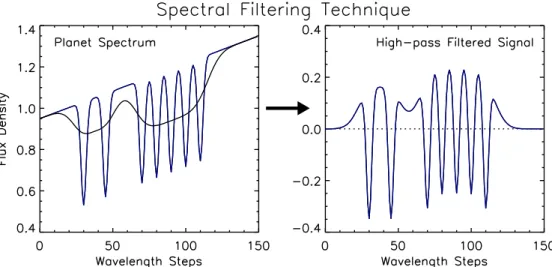
2. A High-pass Spectral Filtering Technique
We argue that the spectralfiltering technique will work well for the MRS mode of MIRI targeting CO2at 15μm. In the case
of Proxima b, its variations in the radial component of its orbital velocity of up to 50 km s−1corresponds to a shift of±1 wavelength step, which may also be detected and subsequently constrain its orbital inclination.
2.1. MRS Mode of MIRI
The MRS mode of the MIRI(Rieke et al.2015; Wright et al.
2015)on JWST utilizes an integralfield spectrograph(IFS)that has four image slices producing dispersed images of the sky on two 1024×1024 infrared detector arrays, which provide R= 1300–3600 integral field spectroscopy over a λ=5–28.3μm wavelength range(Wells et al.2015; Labiano et al.2016). The spectral window is divided into four channels covered by four integral field units: (1)4.96–7.77μm, (2) 7.71–11.90μm, (3) 11.90–18.35μm, and(4)18.35–28.30μm.
Two grating and dichroic wheels select the wavelength coverage within these four channels simultaneously, dividing each channel into three spectral sub-bands indicated by A,B, and C, respectively. To obtain a complete spectrum over the whole MIRI band, one has to combine exposures in the three spectral settings,A,B, andC. As we are primarily interested in the 15μm CO2feature, only one setting will be sufficient: 3B
covering the 13.2–15.8μm range. Note that the same setting will deliver the 1B (5.6–6.7μm), 2B (8.6–10.2μm), and 4B (20.4–24.7μm) wavelength ranges for free. Of these, 2B is particularly interesting because it contains the ozone absorption feature. This is briefly discussed in Section3.5.
The IFS of Channel 3 consists of 16 slices(width=0 39), each containing 26 pixels(0 24)providing afield of view of
∼6″×6″. The spectrum is dispersed over 1024 pixels (1 pix=2.53 nm=52 km s−1) at a spectral resolving power of R∼1790–2640(168–113 km s−1).
2.2. Modeling Proxima b and Its Atmosphere
Exoplanet Proxima b is found to orbit its host star in
11.186 0.002days 0.001
-+ (Anglada-Escudé et al.2016). The amplitude
of its radial velocity variations corresponds to a minimum mass of1.27-+0.170.19MEarth. If the mean density of the planet is the same
as that of the Earth, and its orbit is nearly edge-on, it will have a radius of∼1.1REarth. Proxima Cen has an estimated mass of
0.123±0.006 MSun, implying an orbital semimajor axis of 0.0485-+0.00510.0041au, corresponding to a maximum angular
separa-tion of 37.5 mas. Proxima Cen has an effective temperature of TEff=3042±117 K, radius of 0.141±0.007 RSun, and
bolometric luminosity of L=0.0017 LSun (Doyle &
But-ler1990; Ségransan et al.2003; Demory et al.2009).
Due to the close vicinity of the planet to its host star, it is generally assumed that Proxima b is tidally locked, meaning that the same dayside hemisphere is eternally facing the star. The planet effective dayside temperature will strongly depend on its Bond albedo and global circulation patterns. If, due to atmospheric circulation, the absorbed stellar energy is homo-geneously distributed over the planet, and the Bond albedo is similar to that of Earth (AB=0.306), the dayside equilibrium
temperature of Proxima b is 235 K. If there is effectively no circulation and the absorbed stellar energy is instantaneously reradiated, its observed dayside temperature could be as high as 300 K(and even up to 320 K for a moon-like albedo). In the other extreme case, in which the planet has an albedo comparable to Venus (AB=0.9) with a very effective
atmo-spheric circulation, its dayside effective temperature could be as low as 145 K. For the calculations below, we assume a continuum brightness temperature of 280 K at 15μm and a near-transiting orbital inclination, corresponding to a planet/ star contrast ratio of 6×10⁻⁵at superior conjunction.
Simulated high-resolution emission spectra of Proxima b were generated by the Spectral Mapping Atmospheric Radiative Transfer (SMART) model, assuming it to have an atmosphere such as Earth, using opacities from the Line-By-Line ABsorption Coefficient(LBLABC)tool(both developed by D. Crisp; see Meadows & Crisp1996). The HITRAN 2012 line database (Rothman et al. 2013) was used as input to LBLABC, which generates opacities at ultra-fine resolution (resolving each line with >10 resolution elements within the half-width)on a grid of pressures and temperatures that spans a range relevant to Earth’s atmosphere. Following this, SMART
—which has been extensively validated against moderate- to high-resolution observations of Earth(Robinson et al.2011)—
was used to simulate spectra at 5×10⁻³cm−1 resolution (corresponding to R>105at the simulated wavelengths).
Our spectral simulations used a standard Earth atmospheric model for temperatures and gas mixing ratios (McClatchey et al. 1972), the spectra of which are shown in Figure2. To bound certain extremes in thermal emission, model runs were performed for both clear sky conditions(the“clear atmosphere model”)and for an opaque high-altitude cirrus cloud(located at 0.2 bar, near the tropopause Muinonen et al.1989), called the
“optically thick cirrus model”. Also, to explore a situation with large thermal contrast between the surface and stratosphere, a case where Earth’s stratospheric temperatures were artificially made isothermal and equal to the tropopause temperature (210 K)was simulated (“isothermal stratosphere model”).
2.3. Simulated Observations
First, an estimate of the expected signal-to-noise ratio(S/N) for Proxima Cen with MIRI is obtained from the beta version of theJWSTexposure time calculator.15The 12μm and 22μm flux densities of Proxima have been determined by the NASA Wide-field Infrared Survey Explorer (WISE) to be 924 mJy (mW3=3.838±0.015) and 278 mJy (mW4=3.688±0.025)
respectively, which arefitted to a 3000 K Planck spectrum and subsequently interpolated to 13, 14, and 15μmflux densities of 816, 713, and 630 mJy respectively. Thesefluxes are fed to the exposure time calculator for channel 3B of the MIRI MRS mode. A detector setup of 5 groups and fast readout gives an
integration time of 16.6 s, delivering an S/N of 200 for a total exposure time of 38.85 s. This extrapolates to an S/N of 2000 hr−1 assuming that calibration uncertainties do not contribute to the noise.
The model planet spectra are smoothed to the spectral resolving power ofR=2200(the mean of the MRS 3B band) and subsequently binned to the wavelength steps of the 3B MRS channel. The resulting clear-atmosphere model spectrum normalized by the stellar spectrum (which, for clarity, is assumed to be featureless) is shown in the top panel of Figure 3. Because the spectral filtering technique is only sensitive to the high-frequency signals, the low-frequency components are removed by subtracting a 25 wavelength-step sliding average (a rather arbitrary width) from the spectrum, resulting in the spectral differential spectrum shown in the middle panel. Subsequently, random noise is added to this differential spectrum at a level expected for the total simulated integration time, as shown in the bottom panel of Figure3.
At this stage, it is determined at what statistical significance level the differential model spectrum is preferred to be present in the data with respect to pure noise. This is done by calculating the chi-squared(χ2)of the observed spectrum, with its sliding average and differential model spectrum removed— for a range of planet/star contrasts and radial velocities. The minimumχ2is assigned as the best fit and the Δχ2interval is used to determine the statistical uncertainties of a possible CO2detection. These simulations were repeated for the three
different models, and for a range star/planet contrasts corresponding to different orbital phases or different effective dayside temperatures.
Figure 2.Planet model spectra(see Section2.2)assuming a standard Earth atmospheric model for temperatures and gas mixing ratios, with, on the right, the assumed T/p profile. The upper panel shows the case where the stratospheric temperatures were artificially made isothermal and equal to the tropopause temperature
(isothermal stratosphere model), the middle panel shows a model for clear sky conditions(clear atmosphere model), and the lower panel shows a spectrum for a case with opaque high-altitude cirrus clouds(optically thick cirrus model).
15
3. Results and Discussion
3.1. Detectability
Our simulations show that the 15μm CO2high-passfiltered
signal of the Earth-mass planet can be detected within a limited amount of observing time. The MRS mode of MIRI at the JWST will, in 24 hr integration time (excluding overheads), deliver anR=1790–2640 spectrum of Proxima Cen between 13.2 and 15.8μm at a S/N of ∼10,000 per wavelength step (assuming photon noise). This corresponds to a 1σ contrast limit of ∼1×10⁻⁴. While the high-frequency features in the filtered planet spectrum are typically at a 1–3×10⁻⁵, there are about 100 within the targeted wavelength range—combining to a detection at a ∼2σ level. It means that while the continuum planet/star contrast is at a level of 6×10⁻⁵ (∼0.6σ per wavelength step), the combined spectrally filtered signal over the 3Bband is about a factor of 3–4 higher. The top-right panel of Figure 3 shows the statistical confidence intervals for 5×24 hr of observations if no CO2signal is present, while the
bottom-right panel shows the same, except with the clear-atmosphere CO2model spectrum for a face-on planet injected,
indicating it can be detected at nearly 4σwithin this exposure time. Hence, while the individual CO2features are not visible
in the simulated spectrum, their combined signal can be clearly detected. Results are very similar for the Isothermal Strato-sphere model and the Optically Thick Cirrus model.
3.2. Important Prerequisites
3.2.1. The Stellar Spectrum and Its Variability
We have made several assumptions that are vital for the high-pass spectral filtering technique to succeed in detecting CO2in Proxima b. First, it is assumed that the high-frequency
components of the spectrum of the host star itself are perfectly known. Although low-resolution (R=600) mid-infrared spectra of M-dwarfs taken with the Spitzer Space Telescope (Mainzer et al. 2007) seem featureless, Phoenix model spectra16 (Allard et al. 2012) show that the 13.2–15.8μm wavelength region of an M5V dwarf star harbours thousands of H2O lines, collectively resulting in wavelength-to-wavelength
variations of∼2% in the MIRI MRS spectrum. It means that these features need to be calibrated to better than a relative precision of 1% for them not to interfere with the planet CO2
Figure 3.From model spectrum to simulated MRS MIRI observations assuming the clear-atmosphere model. The top-left panel shows the model spectrum convolved to the resolution of the MRS 3B channel of MIRI, normalized relative to the average starflux. The middle-left panel shows its associated high-pass spectral signal and the lower-left panel with noise added as if Proxima was observed for 5×24 hr. The top-right panel shows the statistical 1, 2, and 3σconfidence intervals when no CO2signal is present, pointing to a 3σupper limit of 50 ppm for the planet/star contrast. The bottom-right panel shows the same, but with the simulated CO2signal
present—detected at∼3.8σ. They-axis indicates the mean planet/star contrast of the(non-spectrallyfiltered)template spectrum between 13.2 and 13.5μm. Note that these simulations assume that both the instrumental spectral response and the stellar spectrum at a wavelength-to-wavelength scale have been determined, which is likely to require extra deep observations at inferior conjunction that serve as a reference(see Section3.2).
16
archival data of Proxima from the UVES spectrograph (R= 100,000)at the VLT separated by 4 days(2009 October 10 and 14)to assess the optical variability of the star. For each of the two nights, a few dozen spectra were combined and the 868–878 nm wavelength range extracted, which is dominated by hundreds of TiO lines but is free of telluric lines. The averaged spectrum was subsequently convolved with a Gaussian to mimic the resolution of MIRI and subsequently binned to match its wavelength steps(inΔλ/λ). After dividing out a linear trend with wavelength, the standard deviation of the ratio of the resulting spectra of the two nights is 4×10⁻⁴. Because these data are possibly limited by flat fielding uncertainties and variability in the mid-infrared is expected to be lower, this result is encouraging.
3.2.2. Instrument Calibration
Another prerequisite is that the spectral responses of the MRS pixels of MIRI can be adequately calibrated. Neither absolute flux calibration nor the low-frequency spectral response are important, but the sensitivity of one wavelength relative to the next is crucial—e.g., the spectral pixel-to-pixel calibration of theflatfield. Potentially challenging is fringing, a common characteristic of infrared spectrometers. It is caused by interference at plane-parallel surfaces in the light-path of the instrument. Experiences with data from ISOandSpitzer show that it can be removed down to the noise level(e.g., Lahuis & van Dishoeck2000). Wells et al.(2015)have characterized the fringing of the MIRI detectors in the laboratory and identify three fringe components with scale lengths(in wave number)of 2.8, 0.37, and 10–100 cm−1, originating from the detector substrate, dichroic, and fringe beating, respectively. The planet CO2 features also show a regular pattern, but with a
characteristic scale length of ∼1.6 cm−1, which fortunately is significantly different from these fringe components. A potentially unwelcome source of error may be fringing in combination with dithering. Small residuals left over after defringing, combined from different dither positions, may be challenging to calibrate.
In the signal-to-noise calculations presented above, we assumed that the instrument calibration is perfect. For it not to add an extra source of noise, the wavelength-to-wavelength precision of theflatfielding and fringe removal must be10−4. If this level can be reached for an individual IFS pixel, a tailored dithering strategy will subsequently push the calibra-tion noise to below 10% of the noise budget for a 24 hr observation. A single observation will have the starlight mostly
In principle, the observations could also be sensitive to other planets in the system. As such planets would likely be in a significantly wider orbit and be colder, the expected signal would be smaller. The CO2signals of such hypothetical planets
could be distinguished from that of Proxima b, as their superior conjunctions would occur on different epochs.
3.3. Phase Variations
A detection of CO2will provide us with both the strength of
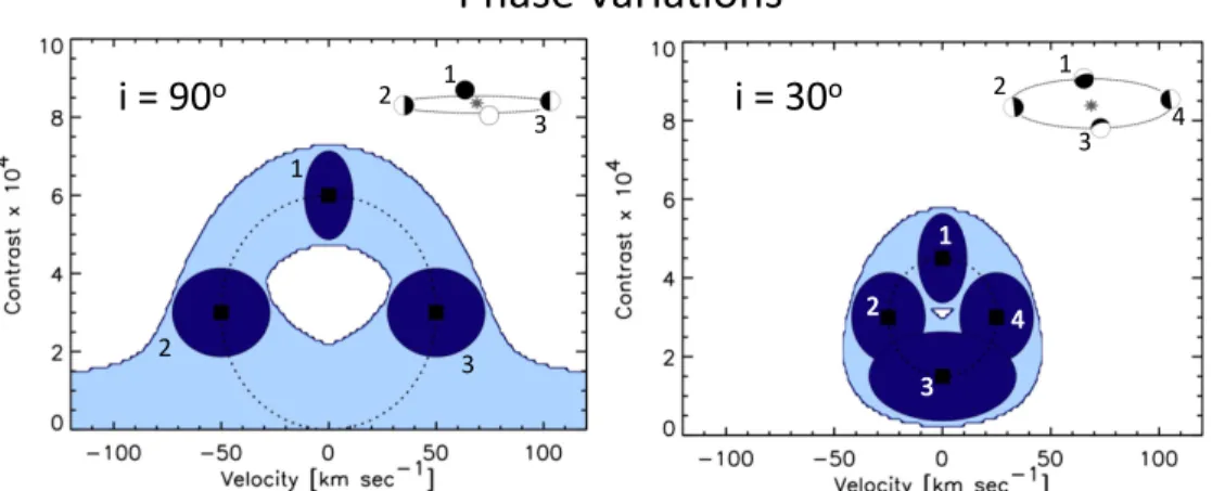
the planet signal and its radial velocity. These can be used to constrain the orbital inclination of Proxima b. An example of such observation is shown in Figure 4, showing, in the left panel, the expected variation in contrast and radial velocity and their uncertainties for 9×24 hr exposures for each three measurements at orbital phase f=0.25, 0.5, and 0.75— assuming an orbital inclination of near 90°. These represent significantly longer exposures than that presented in Figure3. The right panel shows the same, but for an inclination of i=30°, resulting in a smaller variation in contrast and radial velocity as a function of phase. The observations at inferior conjunction may need to serve as a reference for the stellar spectrum(see Section3.2.1). In both cases, it is assumed that all thermalflux originated from the dayside hemisphere of the planet with an effective temperature of 280 K.
Because the strength of the signal atf=0.25 and 0.75 can be up to a factor 2 lower than that atf=0.5, calibration of the instrumental response and the stellar spectrum will be even more important. If the orbital inclination is low, the planet will never be seen entirely face-on, reducing the maximum signal at superior conjunction. However, it would also mean that the mass of the planet is higher, meaning that the planet radius could be larger than assumed above(in particular, if such more massive Proxima b is volatile rich), possibly counteracting the reduction in expected planet surface brightness.
3.4. Atmospheric Characterization
band. This provides an S/N increase of a factor of∼5 over the S/N at at single wavelength step, which can be treated as an upper limit to the differential gain.
Retrieving an injected signal from one model using one of the other spectra results in a significant decrease in signal to noise—not surprising as a large number of the spectral features appear as either emission or absorption in the models. The brightness temperature of the planet atmosphere at a certain wavelength roughly corresponds to the atmospheric temper-ature at the τ=1 surface. In the center of the strongest CO2
lines, where the opacity is greatest, we probe the atmosphere at the highest altitudes. Therefore, in the case of a strong thermal inversion (the clear-atmosphere and the optically thick cirrus models)the atmosphere will be warmer at such low pressure— resulting in emission lines instead of absorption lines when the atmosphere is cooler at higher altitudes. This implies that a detection will also constrain the temperature structure of the upper atmosphere, giving additional insights in high-altitude atmospheric processes. It will not just merely be a detection of the planet atmosphere, which can be compared with theoretical models. For example, Segura et al.(2005)argue that Earth-like planets orbiting M-dwarfs are likely to have relatively cool, bordering-on-isothermal stratospheres—even with O3present.
Several features from other molecules are present in the 13.2–15.8μm wavelength range, such as C2H2at 13.7μm and
HCN at 14μm, which may be included in the atmospheric spectral template if needed(and if expected to be present in the planet atmosphere).
3.5. Prospects of Detecting Ozone
When CO2is targeted in the MRS 3Bband, the 1B, 2B, and
4B bands are observed simultaneously. Interestingly, the 2B band, ranging from 8.6 to 10.3μm covers the 9.6μm ozone band. While CO2 in the atmosphere of Proxima b may be
likely, if the planet did undergo ocean loss early in its history to generate a massive O2atmosphere(Luger & Barnes2015), it is
also possible that O3, photochemically produced from the O2, is
also present in higher abundances than is seen on Earth (Meadows et al.2016). O3is of course also of high interest, as
it can be used as a proxy for the O2 biosignature from a
photosynthetic biosphere. Detection of O3with JWST would
therefore provide an intriguing first hint that life might be present on an extrasolar planet, although O3 production via
abiotic O2from ocean loss would first have to be ruled out.
The expected S/N per wavelength step in a 24 hr observation is 2×10⁴, about a factor of 2 higher than in the 3Bband because of the high stellarflux. On the other hand, the expected continuum planet/star contrast is a factor of∼2 lower compared to that expected at 15μm. Unfortunately, the individual lines within the 9.6μm band are more tightly packed than the lines in the 15μm CO2band, i.e., the ozone
band is not fully resolved at the MRS resolution ofR=2800 in this wavelength range. This means that if ozone is present in the atmosphere of Proxima b, its spectral differential signal will be about a factor of 3–4 smaller than that of CO2. We estimate
that in the best case one could expect a 2σresult in 20 days of JWSTobserving. We also note that the prerequisite for spectral calibration is also more stringent by a factor 2 compared to the CO2case. Hence, although observations of ozone come for free
when the CO2band is targeted, it is unlikely this could result in
afirm detection and is probably beyond the limit of what the JWSTcan achieve.
3.6. Strategy for Proof of Concept and Other Prospects
We envisage two ways to show proof of concept for the high-pass spectral filtering technique with the MRS mode of MIRI. First, the method can be used on exoplanet targets with significantly higher planet/star contrasts. For example, a T=1000 K hot Jupiter orbiting a solar type star will have a 15μm contrast of 10−3, a factor 20 higher than Proxima b. It means that for a host star whose 15μm flux is 40 times (4 magnitudes) fainter than Proxima b, CO2 will still be
detected 10×faster. Also, one could aim for cool Neptunes or super-Earths orbiting nearby M-dwarfs, such as Gliese 687b. If the spectrum of this particular planet exhibits a CO2absorption
feature, it can be detected at a factor of 4 faster than in the case of Proxima b. From a theoretical point of view, it will be important to identify those planets that are expected to have CO2 in their atmospheres and select those with the most
favorable stellar magnitudes and planet/star contrasts. Ultimately, one should target Proxima itself, gradually increasing the integration time and validating at each step that
Figure 4.Examples of phase variation observations of the 15μm CO2feature of Proxima b. The left shows the expected variation for an edge-on orbit, with the light
blue regions indicating the 1σconfidence interval for a 9×24 hr observation at a given orbital phase(hence, nearly 650 hr of observations in total—significantly more than the simulations presented in Figure3). The three dark-blue regions indicate the 1σconfidence intervals for particular observations at an orbital phase of
″–
implying that an Earth-sized planet in the habitable zone ofαCen A could possibly be detected in 24 hr. Unfortunately,αCentauri A will saturate the MIRI detectors within a small fraction of a second, irreversibly damaging the instrument. Possible ways to mitigate this issue need to be investigated.
I.A.G.S. acknowledges funding from the European Research Council (ERC) under the European Union’s Horizon 2020 research and innovation programme under grant agreement No. 694513, and from research program VICI 639.043.107, which is financed by The Netherlands Organisation for Scientific Research (NWO). J.-M.D. acknowledges funding from the European Research Council (ERC) under the European Union’s Horizon 2020 research and innovation programme (grant agreement nr 679633; Exo-Atmos). T.R. and J.L.B. gratefully acknowledge support from the National Aeronautics and Space Administration(NASA)through the Sagan Fellow-ship Program executed by the NASA Exoplanet Science Institute. Support for this work was provided in part by NASA through Hubble Fellowship grantHST-HF2-51336 awarded by the Space Telescope Science Institute, which is operated by the Association of Universities for Research in Astronomy, Inc., for NASA, under contract NAS5-26555. V.M. and T.R. are members of the NASA Astrobiology Institute’s Virtual Planetary Laboratory Lead Team, supported by NASA under Cooperative Agreement No. NNA13AA93A.
ORCID
I. A. G. Snellen https://orcid.org/0000-0003-1624-3667
T. Robinson https://orcid.org/0000-0002-3196-414X
V. Meadows https://orcid.org/0000-0002-1386-1710
C. Dominik https://orcid.org/0000-0002-3393-2459
J. L. Birkby https://orcid.org/0000-0002-4125-0140
M. Brogi https://orcid.org/0000-0002-7704-0153
Kite, E. S., Gaidos, E., & Manga, M. 2011,ApJ,743, 41
Kopparapu, R. K., Ramirez, R., Kasting, J. F., et al. 2013,ApJ,765, 131
Kreidberg, L., & Loeb, A. 2016,ApJL,832, L12
Labiano, A., Azzollini, R., Bailey, J., et al. 2016,Proc. SPIE,9910, 99102W
Lahuis, F., & van Dishoeck, E. F. 2000, A&A,355, 699
Lammer, H., Lichtenegger, H. I. M., Kulikov, Y. N., et al. 2007,AsBio,7, 185
Lovelock, J. E. 1965,Natur,207, 568
Lovis, C., Snellen, I., Mouillet, D., et al. 2017,A&A,599, A16
Luger, R., & Barnes, R. 2015,AsBio,15, 119
Luger, R., Lustig-Yaeger, J., Fleming, D. P., et al. 2017,ApJ,837, 63
Mainzer, A. K., Roellig, T. L., Saumon, D., et al. 2007,ApJ,662, 1245
McClatchey, R. A., Fenn, R. W., Selby, J. E. A., Volz, F. E., & Garing, J. S. 1972, Optical Properties of the Atmosphere(3rd ed.; Bedford, MA: Air Force Cambridge Research Laboratories(OP))
Meadows, V. S., Arney, G. N., Schwieterman, E. W., et al. 2016, arXiv:1608. 08620
Meadows, V. S., & Crisp, D. 1996,JGR,101, 4595
Muinonen, K., Lumme, K., Peltoniemi, J., & Irvine, W. M. 1989,ApOpt,
28, 3051
Ramirez, R. M., & Kaltenegger, L. 2014,ApJL,797, L25
Reynolds, R. T., Squyres, S. W., Colburn, D. S., & McKay, C. P. 1983,Icar,
56, 246
Riaud, P., & Schneider, J. 2007,A&A,469, 355
Ribas, I., Bolmont, E., Selsis, F., et al. 2016,A&A,596, A111
Rieke, G. H., Wright, G. S., Böker, T., et al. 2015,PASP,127, 584
Robinson, T. D., Meadows, V. S., Crisp, D., et al. 2011,AsBio,11, 393
Rodler, F., & López-Morales, M. 2014,ApJ,781, 54
Rothman, L. S., Gordon, I. E., Babikov, Y., et al. 2013,JQSRT,130, 4
Ségransan, D., Kervella, P., Forveille, T., & Queloz, D. 2003,A&A,397, L5
Segura, A., Kasting, J. F., Meadows, V., et al. 2005,AsBio,5, 706
Snellen, I., de Kok, R., Birkby, J. L., et al. 2015,A&A,576, A59
Snellen, I. A. G., Brandl, B. R., de Kok, R. J., et al. 2014,Natur,509, 63
Snellen, I. A. G., de Kok, R. J., de Mooij, E. J. W., & Albrecht, S. 2010,Natur,
465, 1049
Snellen, I. A. G., de Kok, R. J., le Poole, R., Brogi, M., & Birkby, J. 2013,ApJ,
764, 182
Sparks, W. B., & Ford, H. C. 2002,ApJ,578, 543
Tarter, J. C., Backus, P. R., Mancinelli, R. L., et al. 2007,AsBio,7, 30
Turbet, M., Leconte, J., Selsis, F., et al. 2016,A&A,596, A112
Venot, O., Rocchetto, M., Carl, S., Roshni Hashim, A., & Decin, L. 2016,ApJ,
830, 77
Wells, M., Pel, J.-W., Glasse, A., et al. 2015,PASP,127, 646