Genetic Algorithms for Auto-tuning Mobile Robot Motion Control
Chris Messom
Institute of Information and Mathematical Sciences,
Massey University, Albany Campus, Auckland, New Zealand
[email protected]
Abstract
This paper discusses a genetic algorithm (GA) based method for automatically tuning mobile robot motion controllers. The genetic algorithm evolves a controller that is optimised for a given performance measure. Genetic algorithms require a mapping from the genetic code to an implementation. This translation between the chromosome and the implementation allows the use of standard GA libraries, however the assumption constrains the types of problems that can be solved.
1. Introduction
Mobile robot path planning and motion control has tended to be treated independently in the literature [1]. Path planning is often a slow process that assumes that the current state of the world is static and that the time taken to create the plan will not have significant effects on the performance of the robot [2]. Motion control in contrast assumes that a path plan exists and that the motion controller has to follow the plan as closely as possible. This divide and conquer approach has produced many sophisticated techniques for path planning and control that are however difficult to implement in a real systems. Real-world mobile robot systems, such as robotic pets, hospital automatic guided vehicles (AGV) etc, are required to operate in environments with fast moving unknown obstacles.
Combining the path planning and motion control approaches in a fast dynamic environment tends to be detrimental to the robot and its environment as the path planned does not reflect the current state of the world. Several authors adopt a simple path planning approach which identifies only the target position of the robot and passes the obstacle avoidance to the motion control layer using techniques based on a vector field approach [3]. In a dynamic environment the vector field must be frequently recalculated, however this need not be too computationally intensive in an environment with few obstacles. The main disadvantage with vector field based approaches is that they are ideal for static obstacles but tend to produce poor performance in dynamic environments. This can be illustrated with the example of the problem of crossing a road. Given a road with fast moving cars it is easier to cross the road by planning a path that predicts the movement of the obstacles (the cars) and then just cross the road at the right time. If a vector field approach is adopted the robot will be pulled towards the goal when there is a gap in the traffic while repelled by a nearby obstacle. The unknown or uncertain dynamics of vector field will make the robot movement unpredictable and dangerous. It will be very difficult to tune the vector field so that the robot motion becomes reliably safe for obstacles moving at different speeds.
2.
Mobile Robot Kinematics
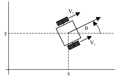
The mobile robot model used for the experiments is a kinematic model of a two-wheeled mobile robot. The mechanical structure is configured in a wheel chair format. The robot is controlled by assigning velocity set points for the left and right wheels, there is no separate steering wheel. The kinematic model is given in equation 1
The distance between the robot wheels is d, Vl and Vr are the left and right wheel velocity set points, (x,
[image:2.595.74.271.337.469.2]y) is the position of the robot and θ is the angle of the robot. The system variables are illustrated in figure 1.
Figure 1. The mobile robot system variables
3.
Genetic Algorithm System
The genetic algorithm system was used to auto-tune a gain-scheduled controller. The gain schedule controller had 11 gain values for the angle error and 7 gain values for the distance error. The angle error gains are for the ranges π - 3π/4, 3π/4 - π/2, π/2 - π/4, π/4 - π/8, π/8 - π/16, π/16 - -pi/16, -π/16 - -π/8,
-π/8 - -π/4, -π/4 - -π/2, -π/2 - -3π/4, -3π/4 - -π. The distance error gains are for the ranges ∞ - 50, 50 - 35, 35 - 25, 25 - 15, 15 - 10, 10 - 5 and 5 - 0. It is expected that the angle gains will be symmetric about zero but the controller is free to evolve nonsymmetric gains if these produce an optimal controller over the training set of data. The controller provides the required velocity set point to the left and right wheels via the control formulae given in equation 2.
VL = Kd.distanceError + KA.angleError
VR = Kd.distanceError - KA.angleError
The distanceError variable is the distance of the robot to the target, while the angleError variable is the angular difference between the heading of the robot and the vector from the robot to the target. Kd is the
scheduled gain for the given distance error and KA is the scheduled gain for the given angle error.
The population size used for the genetic algorithm was 40 while the number of generations was 20. Each individual consisted of the 11 KA gains and 7 Kd gains. Each gain was coded as a 20 bit precision gene.
Each individual was evaluated with 20 random test positions taken from various regions around the goal
dx/dt
dy/dt
dθ/dt 1 0 0
0 1 0
0 0 d/2π
Vl
Vr
_ cos(θ) _ cos(θ)
_ sin(θ) _ sin(θ)
-1/2 1/2
y
x
θ
Vr
Vl
(1)
position. The cost function was the sum of the distances of the robot from the target position after running a kinematic simulation of the 20 test positions.
The 20 test cases do not cover all the possible regions of the input space (7 * 11) but the performance of the controller is likely to be effected by all the gain values. Also since each individual is re-evaluated at each generation, solutions that are unfit for a particular initial region are unlikely to occur.
3.1 Genetic algorithm operators
The initial population is generated with small random numbers. Each individual's chromosome consists of 360 bits ((11+7)*20 bits). Although this chromosome consists of 18 different 20-bit precision floating point numbers they are not represented by 18 genes but rather as 360 one-bit genes that can then be genetically manipulated. The detail of how these genes are expressed in the performance measure is not directly available to the genetic algorithm engine.
The genetic operators that were applied to this system are ranking based selection, single point crossover and genetic mutation. Individuals are selected from the population for reproduction based on their fitness values. The fitter individuals are the ones with the least cost, that is, individuals that get closest to the target position. The population is ranked based on the fitness of the individuals and this ranking is used to select individuals for crossover. When two individuals have been selected single point crossover randomly selects a position in which to split the chromosomes and swaps the two individuals' genes. This is illustrated in figure 2 for two 9-bit chromosomes with the crossover point between the 4th and 5th gene.
Figure 2. Single point crossover
Mutation is the process of selecting an individual gene and changing its value. In this example each gene consists of a single bit, so the only change that mutation can introduce is to toggle a bit from 0 to 1 or from 1 to 0. Mutation is included as an operator to recover a gene that may have been lost in the population. It is not the primary operator in the algorithm, which is reflected in the low probability (0.001) of mutation. The fast convergence of this example (see section 4) indicates that it is unlikely that mutation played a significant part in the convergence. However for some randomly selected inititial population, mutation may be the only genetic operator that ensures convergence.
4. System Performance
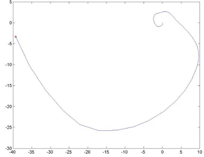
Figure 3 shows the convergence of the best of each generation. It can be seen that there is rapid convergence within 10 generations to an almost perfect solution. The remaining generations produce minor variations as the algorithm continues to optimise the controller over the test cases. Figure 4 shows an example test run of the best of generation individual after the 20 generations of learning. The performance is good, the robot reaches the target position within the simulation time. However the performance is not optimal over all possible input values as the evaluation function did not exhaustively test the possible input space.
Chromosome 1:110010100 Chromosome 2:111110111
New Chromosome 1:110010100 New Chromosome 2:110010100
Crossover point
Figure 3. Convergence of performance algorithm
The example also illustrates the difficulty of designing a good evaluation function. The robot approaches the target position exactly as the simulation time comes to an end. In a real system we would normally require the robot to reach the target position as fast as possible. The choice of evaluation function used will often influence the performance of the final solution in unexpected ways. The controller design load moves from actually designing the controller to developing evaluation functions that will lead to solutions that exhibit the behaviour required.
Figure 4. x,y plot of robot position from a random start point to the 0,0 endpoint
5.
Discussion
[image:4.595.75.281.400.559.2]5.1 Application to real robot control
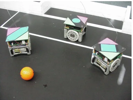
Using genetic algorithms to develop real robot controllers by applying a large population and a large number of test cases is impractical since each test case will be very time consuming and provide significant wear and tear on the robot. See figure 5 for the mobile robot model. For example the population of 40 controllers run for 20 generation on a test set of 20 random start points with each experiment running for 5 seconds will require approximately 22 hours of continuous run time. This does not include the set up time to move the robot to the start position, which may exceed 5 seconds and the time to change and recharge the batteries.
[image:5.595.114.345.279.452.2]An alternative approach is to use the genetic algorithm to auto-tune the controllers, offline, on a kinetic and then a dynamic model before transferring the controller to a real system for fine-tuning. Given a favourable initial condition it is expected that the number of generations required to converge to a suitable solution will be reduced to the point that it will become feasible.
Figure 5. Mobile Robot Model
6.
Conclusions
References
[1] Huang Q., Yokoi, K, Kajita, S, Kaneko, K, Arai, H, Koyachi, N, and Tanie, K, "Planning Walking Patterns for a Biped Robot", IEEE Transactions on Robotics and Automation, June 2001, vol 17, number 3, pp 280-289.
[2] Baltes J. and Lin Y.M., "Path Tracking Control of a Non-holonomic Car-like Robot with Reinforcement Learning", RoboCup-99: Robot Soccer World Cup III, Springer Verlag, 2000, pp162- 173.
[3] Arkin, R. and Murphy, R.R., "Autonomous Navigation in a Manufacturing Environment", IEEE Transactions on Robotics and Automation, vol 6, no 4, 1990, pp 445-454.
[4] Holland J.H., "Adaptation in Natural Artificial Systems", University of Michigan Press, 1992.
[5] De Jong, K., "Learning with Genetic Algorithms: An Overview", Machine Learning-3, pp 121-138, Kluwer Academic Publishers, 1988.
[6] Chin T.C. and Qi, X.M, "Integrated Genetic Algorithms based Optimal Fuzzy Logic Controller Design", Proceedings of the Fourth International Conference on Control, Automation, Robotocs and Vision, 1996, pp563-567.
[7] Lee, C., "Genetic Algorithms for the Control of the Inverted Pendulum", unpublished MSc Thesis, Department of Automatic Control and System Engineering, University of Sheffield, 1995.