ANALYTICAL AND NUMERICAL STUDIES ON STRATIFIED FLUID FLOWS
by Claudio Viotti
A dissertation submitted to the faculty of the University of North Carolina at Chapel Hill in partial fulfillment of the requirements for the degree of Doctor of Philosophy in the Department of Mathematics.
Chapel Hill 2012
Approved by:
Roberto Camassa Richard M. McLaughlin
David Adalsteinsson M. Gregory Forest
c
2012
Claudio Viotti ALL RIGHTS RESERVED
Abstract
CLAUDIO VIOTTI: ANALYTICAL AND NUMERICAL STUDIES ON STRATIFIED FLUID FLOWS.
(Under the direction of Roberto Camassa and Richard M. McLaughlin.)
The mathematical modeling of stratified fluid flows is the overall subject of this work, which spans a range of more specific topics: internal gravity waves, shear in-stability, anomalous diffusion of passive scalars, vortex rings dynamics in stratified environments. This dissertation is organized in three parts.
Part I focuses on shear-induced instability in large amplitude internal waves. Pre-vious studies have shown that an instability of the Kelvin–Helmholtz type can occur within internal wave-induced shear layers, leading to wave breaking and production of turbulence. It was also recognized that such wave breaking resembles the instability of parallel shear flows only superficially. This study aims to refine the understanding of shear-induced instability in this specific context, and to identify the mechanisms that eventually make the onset of shear instability for such flows a significantly more subtle mechanism than its parallel counterpart.
Part II is concerned with anomalous diffusive regimes for passive scalars advected in shear flows. The problem is studied from the standpoint of spectral analysis, which provides a natural way to classify diffusive regimes ensuing from different asymptotic limits in the governing parameters. The analysis identifies separate classes of eigen-modes, whose features dominate the evolution at different time and space scales in initial value problems with multiscale initial conditions.
environ-Fluid Lab. Vortex rings made of fluid with density higher than the ambient fluid and propagating downward through a sharp density stratification are considered. Lab experiments have identified a critical phenomenon, which distinguishes the behavior of the falling vortex ring in either being fully trapped at the ambient density layer, or continuing through the layer in its downward motion. The numerical simulations presented are able to reproduce such behaviors and offer several details not visible in experiments.
Acknowledgments
I am indebted to several persons who contributed to my work. I thank Roxana Tiron, for handing to me the internal wave project, supplemented with useful tools that I used throughout my work. I thank David Adalsteinsson, for providing the DataTank software and for his kind assistance. I thank Ann Almgren, for providing the VARDEN–Boxlib Navier–Stokes solver and for all the help. I thank Keith Mertens and Shilpa Khatri for their collaboration in the vortex ring project.
I thank my advisors, Roberto Camassa and Rich McLaughlin, from whom I have learned a great deal of science, and who made the years of graduate school a rewarding and pleasant experience.
I dedicate this thesis to my wife Martina. She has been my support and inspiration through all these years.
Table of Contents
List of Figures . . . xi
I STABILITY OF PARALLEL AND WAVE-INDUCED NON-PARALLEL STRATIFIED SHEAR LAYERS . . . 1
1 Introduction . . . 2
1.1 Internal gravity waves . . . 2
1.2 Shear instability in large-amplitude internal waves . . . 4
1.3 Mathematical modeling of non linear internal waves . . . 6
1.3.1 Governing equations . . . 6
1.3.2 Reduced models . . . 7
1.4 Solitary waves . . . 9
1.4.1 DJL equation . . . 10
1.4.2 Green-Naghdi solitary waves . . . 11
2 Spectral analysis of stratified parallel shear flows: well and not-so-well known facts . . . 13
2.1 The Taylor–Goldstein equation . . . 14
2.1.1 Discrete spectrum . . . 16
2.1.2 Continuous spectrum . . . 19
3 Local spectrum along a wave-induced non parallel shear . . . 21
3.1 Model for the internal wave structure . . . 22
3.1.1 Three-layer configuration . . . 22
3.2 Computation of the local spectrum . . . 26
4 Response of large amplitude internal waves to upstream perturbations . . . 33
4.1 Problem setup . . . 35
4.1.1 Single baroclinic mode disturbance of internal solitary waves prop-agation . . . 35
4.2 Numerical simulations . . . 39
4.2.1 Energetic diagnostics . . . 41
4.2.2 The parallel shear case . . . 47
4.2.3 Self-induced shear by internal waves: the locally stable case . . 50
4.2.4 Self-induced shear by internal waves: the locally unstable case . 52 4.2.5 Interpretation in terms of spatial spectrum . . . 56
4.3 Discussion of results . . . 61
5 Continuous spectrum and non-normal transient dynamics . . . 63
5.1 Singularities of the continuous spectrum eigenfunctions . . . 65
5.2 Continuous-spectrum solutions . . . 67
5.2.1 Temporal solutions . . . 69
5.2.2 Spatial solutions . . . 72
5.3 Numerical verification . . . 74
5.3.1 Computational issues . . . 75
5.4 Discussion . . . 77
II ANOMALOUS DIFFUSIVE REGIMES OF PASSIVE
TRACERS IN SHEAR FLOWS . . . 80
6 Introduction . . . 81
7 WKBJ analysis for advection-diffusion problems . . . 84
7.1 The advection-diffusion eigenvalue problem . . . 86
7.1.1 Exact estimates on λ . . . 87
7.2 WKBJ solutions in the complex plane . . . 88
7.2.1 Wasow theorem and connection formulas . . . 90
7.3 Computing eigenvalues using WKBJ: asymptotic matching . . . 93
7.4 Variants of WKBJ analysis in specific cases . . . 97
7.4.1 Sawtooth shear flow . . . 97
7.4.2 Cellular flow . . . 104
8 Sorting of eigenmodes at intermediate time scales . . . 108
8.1 Outline . . . 108
8.2 Three classes of modes . . . 110
8.2.1 The limit ǫ→ ∞: Taylor modes . . . 111
8.2.2 The limit ǫ→0: anomalous modes . . . 112
8.2.3 The limit ǫ→0,k ≫P e1/3: pure-diffusive modes. . . 121
8.2.4 Poiseuille flow: global view of the spectrum . . . 122
8.3 Initial value problems . . . 124
8.3.1 Single-scale initial data . . . 125
8.3.2 Multi-scale initial data . . . 129
8.4 Concluding remarks . . . 138
III NUMERICAL SIMULATIONS OF DENSE-CORE
VORTEX RINGS IN A SHARPLY STRATIFIED ENVIRONMENT . . . 140
9 Dense-core vortex rings in a sharply stratified environment . . . 141
9.1 Introduction . . . 142
9.2 Brief description of lab experiments . . . 146
9.2.1 Critical phenomena: entrapment versus escape . . . 148
9.3 Governing Equations . . . 149
9.4 Numerical Method . . . 152
9.4.1 Initial conditions . . . 152
9.4.2 The initial condition problem for the simulations . . . 154
9.5 Simulations . . . 155
9.5.1 Vortex ring dynamics: homogeneous environment . . . 156
9.5.2 Vortex ring dynamics: stratified environment . . . 157
9.5.3 Some comments about resolution effects . . . 159
9.6 Discussion . . . 160
A Slow-varying media asymptotics for weakly non-parallel stratified shear flows (appendix to Part I) . . . 162
A.1 Multiscale method in weakly non-parallel stratified flows . . . 167
A.2 Details of the derivation . . . 173
A.2.1 Continuous part: stability operators . . . 173
A.2.2 Discrete part: interface conditions . . . 177
A.3 A few useful relations . . . 182
A.3.1 Computing Ωk and ΩX from eigenfunctions . . . 182
B Scalar variance evolution from Taylor modes
(appendix to Part II) . . . 185
B.1 Problem Formulation . . . 186
B.2 Eigenvalue problem, perturbative analysis . . . 187
B.3 Longitudinal dispersion . . . 190
B.3.1 Channel flow with transversely uniform data . . . 191
B.3.2 Pipe flow with transversely uniform data . . . 193
Bibliography . . . 195
List of Figures
1.1 Schematics of the two-fluid system with main notation definitions. . . . 8 1.2 Comparison between a solitary wave in a continuous sharp stratification
and a Green–Naghdi solitary waves that matches the maximum displace-ment of the mean-density isoline. Such isolines are referenced by the blue (continuous stratification) and red-dashed (Green–Naghdi) lines. The solitary wave in continuous stratification is computed using the TEW algorithm, the grayscale map represents the corresponding density field. The background stratification is set as described later in §4.1.1, with
ρ1 = 1, ρ2 = 1.02 and δ = 1/16. The wave speed is cW = 0.212, which corresponds to a wave approaching the propagating front limit. . . 13 2.1 Deformation of the integration contour for computing eigenfunctions
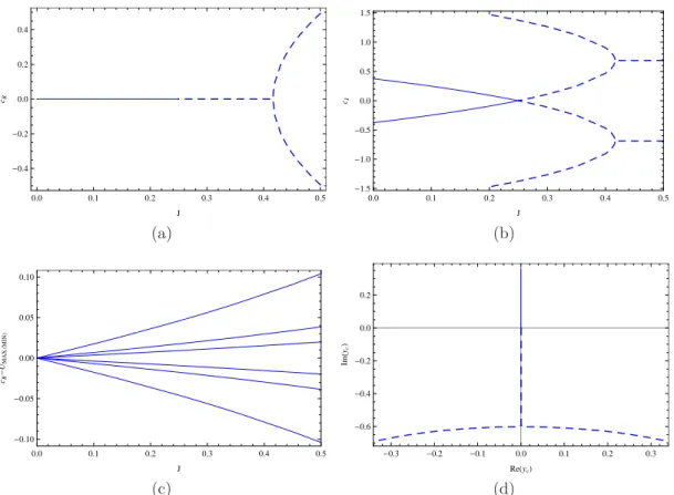
of (2.3) in the complexified y-plane as the branch point yc crosses the real axis, going from unstable (left panel) to stable (right panel). . . . 17 2.2 Spectrum calculations for k = 0.5. (a) cR for the unstable mode; (b) cI;
(c) realcfor a few neutral modes. All eigenvalues are plotted against the overall Richardson number. (d) locus in the complex plane of the branch point yc corresponding to the unstable eigenvalue as J is varied. The lines are dashed after the branch point crosses the real axis (unphysical modes). . . 18 2.3 Eigenfunctions computed on the tanh shear layer in a bounded domain,
all computed for k = 1. The overall Richardson number is J = 0.35 (no complex spectrum). Rigid-lid boundary conditions are applied at the domain boundaries y = ±6. Left plot: three pairs of continuous spectrum modes, ˆφ+ (solid lines) and ˆφ− (dashed lines). Right plot:
first three pairs of discrete spectrum modes, ˆψn, corresponding to the three largest eigenvalues cn > Umax (solid lines) and the three smallest
cn< Umin (dashed lines). . . 21
2.4 Real and imaginary parts of the unstable mode eigenfunction. Computed on the tanh shear layer in a bounded domain, for k = 0.5 and J = 0.1. Rigid-lid boundary conditions are applied at the domain boundaries y=
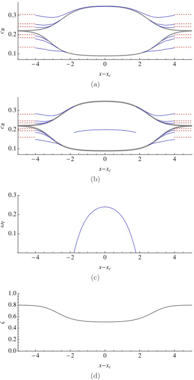
3.3 Local eigenvalues computed on the background flow model as a function of x−xc, withxc = 8. (a) Phase speedcRfor the W1 wave, with k =kB for run W1R (or equivalently W1L). The branches continuing the first 6 baroclinic modes are shown. Grey-thick curves are the velocity extrema
U1 andU2 from the model (recallU2 > U1). (b) Similar plot for wave W2 (thinner pycnocline), withk=kBfor run W2L1 (or equivalently W2R1). An unstable mode develops near x = x0. (c) Growth rate ωI = kcI for the unstable mode. (d) Wave profile represented by ζ(x). The |x| → ∞
limiting values for cR are reported in (a) and (b) (dashed lines). . . 30 3.4 Horizontal velocity (a)–(c) and density (b)–(d) profiles at the wave’s
maximum reconstructed from the model (dashed lines) versus the full numerical computations (solid lines). Pycnocline thickness δ= 0.1 (a)– (b) and δ= 0.05 (c)–(d) . . . 31 3.5 Eigenvalues computed from the model (circles) versus the computations
based on the actual profiles (diamonds) from the DJL numerical solution. The real eigenvalues correspond to the first and second neutral mode of the family approaching U1+ at the wave maximum, for δ = 0.1, the complex ones are the unstable mode for δ = 0.05. . . 32 4.1 Simulation of an internal wave interacting with a train of upstream
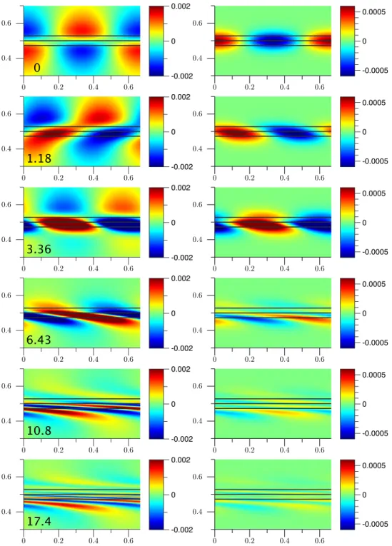
perturbing mode-1 baroclinic waves. The horizontal velocity compo-nent of the perturbation is depicted, internal labels denote the time instants. This is case W1R in table 4.1, full discussion in §4.2. La-bels correspond to time, and the pycnocline is referenced by two iso-lines (R = 1.005,1.015) of the basic state density (varying in the range 1≤R ≤1.02). The domain shown is full-extent in the vertical, but only a center subsection of the domain is shown in the horizontal. The area inside the box is magnified in figure 4.5. . . 38 4.2 Schematic of the energy transfer across the four constituent parts of
the total energy. Our convention for the sign of the transfer terms is indicated by the arrows. The solid-line connections mark the transfers allowed in parallel shears. . . 45 4.3 Horizontal velocity perturbation (left) and density perturbation (right)
from parallel shear simulation. The lines reference the same levels of background density as in figure 4.1 (R = 1.05,1.015), the labels inside left panels indicate time. . . 46
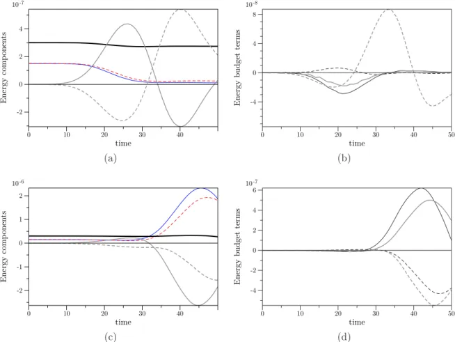
4.4 (a) Time evolution of integrated energy components computed from nu-merical simulations for the parallel-shear background. The curves are:
hEKi solid-blue, hEAi dashed-red, heKi solid-grey, heAi dashed-grey,
to-tal sum solid-black-thick. (b) Volume-integrated energy budget terms versus time. The curves are: PK solid-black, PA dashed-black, CE
KtoA
solid-grey,Ce
KtoAdashed-grey, andPK−CKtoAE dash-dot. Markers are the
time-derivatives of hEKi and hEAi computed through interpolation.
No-tice thatheAi,PA, andCe
KtoA are identically null in this case (line-styles
are given for future reference). . . 47 4.5 Blow-up of the region near the maximum slope of the pycnocline for the
snapshots in figure 4.1, showing (a) horizontal velocity and (b) density perturbations. Notice the different times (labeled in panel (a)) with respect to figure 4.1 to better zoom in on the entrainment phase. . . 49 4.6 Same as figure 4.4, but for run W1R. . . 49 4.7 Instability pocket (Ri < 1/4 region) for the locally unstable wave W2.
The color map represents the local value of Ri, the dashed line is the isoline R = 1.01. Notice the bias of the pocket towards the upper layer for this wave. . . 52 4.8 Same as figure 4.1 now for runs W2R1 (a) and W2L1 (b) in table 4.2.
Notice that unstable growth takes place only in case (b). . . 53 4.9 Same as figure 4.4, now with non-parallel shear background flow from
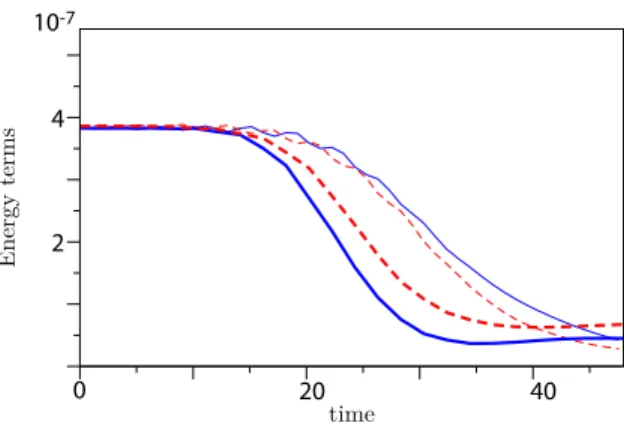
W2 wave. (a),(b) W2R1 (c),(d) W2L1. Note the different scales between the plots. . . 54 4.10 Pertubation energy for runs W1R and W1L (thicker lines). Solid lines
are hEKi, dashed lines are hEAi. . . . 56
4.11 Dispersion relations (in the wave frame) for the first pair of baroclinic modes of the far-field undisturbed stratification ¯ρ(y). Markers corre-spond to the modes used in different runs. . . 57 4.12 Spatial spectrum at the wave maximum as a function of ω. Solid line
is kR, dashed line kI. The vertical lines reference the perturbation fre-quencies in runs W2R2-W2L1 (left) and W2R1-W2L2 (right). . . 57 4.13 Direct comparison of perturbation growths for all runs using the W2
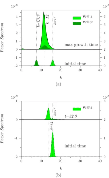
4.14 (a) Fourier power spectra of the 1-dimensional signal obtained by evalu-ating ρ′ along the isopycnal R = (ρ1+ρ2)/2, taken at t = 0 and at the
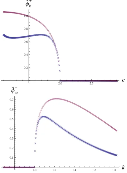
time corresponding to the maximum amplification for each run. (b) Sim-ilar plot for run W2R1. The isopycnal is displaced downward,R = 1.017, to better focus on the features of interest (cf. discussion) . . . 59 5.1 Examples of continuous spectrum modes (blue symbols) compared to the
leading order Frobenius expansions (purple symbols) given by (5.6) and (5.7). Eigenfunctions ˆφ+k(y, c) (top) and ˆφ+
ω(y, k) (bottom) as a function of c and k respectively, for y= 0. . . 67 5.2 Regions in the (c, k) and (ω, k) spaces filled by the
continuous spectrum. . . 68 5.3 Path of integration for ˆφ+-mode solution. . . . 71
5.4 Time frames of a ˆΦk solution with w+=e−8(yc(c))2
,w−= 0
and k= 2/3. . . 74 5.5 A ˆΦω solution withw+=e−8(yc(ω/k)+1/2)2
,w−= 0 and ω= 2. Top panel
shows streamfunction, bottom panel density. For the background shear parameters see the caption of figure 2.3. . . 74 5.6 Comparison between “exact solutions” constructed numerically
(mark-ers) and the asymptotic expansions (lines). Left panel: time evolution of the temporal solution reported in figure 5.4 taken at x = 0 and
y =−0.33. Right panel: horizontal slice of the spatial solution reported in figure 5.6 taken at y =−0.57 andt = 0. . . 75 5.7 Demonstration of time-periodic behavior for a spatial solution in a full
numerical simulation using VARDEN. It is shown the time evolution of an horizontal slice of the density field taken aty = 0. The portion shown corresponds to −14 < x < 14 and 0 < t < 18.8, which spans about 6 periods with ω = 2. . . 76 5.8 Sketch of the spectrum excited by an upstream perturbation illustrating
the hypothesis of energy leak on the continuous spectrum (which lies in the entire area enclosed between the thick gray curves representing the velocity extrema). The picture is based on a replica of figure 3.3b, which contains the eigenvalue branches (real part) along a wave-induced shear layer. See the referred plot for further details. . . 79 7.1 Domains of validity of the three asymptotic solutions wk. . . 91 7.2 In S1∪µ2∪ S3 the functionw1 can be interchanged with γw2+δw3, the
second one however gives uniform asymptotics in this set. . . 93
7.3 Stokes (dashed) an anti-Stokes (continuous) lines for turning-points close to the origin. The shaded region is the (open) set S. . . 95 7.4 Ground-state mode for the cellular flow (ǫ= 10−3). . . 105
7.5 Sketch of the Stokes lines emanating from r0. . . 106 8.1 Ground-state mode for ǫ = 10−3 (k = 0, Pe = 1000), comparison
be-tween cosine u(y) = cos(y) and sawtooth u(y) = 1 − |y| shear pro-files, respectively top and bottom pictures. For the cosine flow case the eigenfunction is constructed using Hermite uniform asymptotic approx-imation, for the sawtooth it is computed exactly using Airy functions (discussed in the text). . . 117 8.2 Snapshots of the time evolution governed by (7.1) withu(y) = 1−4(y−
1/2)2 and P e = 103, from the initial condition T0(x, y) = exp(−(x− Lx/2)2/ℓ2x), withℓx = 10−3/2Lx, and horizontal Fourier periodLx = 20π, with nx = 1024 and ny = 128 respectively for horizontal and vertical Fourier modes. Snapshots are taken at t = 0,7,16,27 from top to bot-tom. Neumann boundary conditions Ty(0) =Ty(1) = 0 are enforced, by even symmetry with respect to the y = 0 and y = 1 horizontal bound-aries. The localization of the tracer near the walls and the center of the channel is evident, as are the different speeds and decay rates for these two regions, (the peaks are normalized by the scalar’s maximum). . . . 120 8.3 Schematics of the periodic extension for channel flow: support of interior
and wall modes is determined by the scaling of the imaginary part of the eigenvalues of cosine and linear shear, respectively. . . 121 8.4 Position of the tracer distribution peak near the wall for the simulation
depicted in figure 8.2 compared to the wall-mode theoretical prediction for the phase speed based on the characteristic wavenumber of the initial condition (k ≃π for the initial data in the simulation). . . 122 8.5 Exact eigenvalues for plane Poiseuille flow, cosine flow and sawtooth
flow versus wavenumber k, for Pe= 1000. Top panels: eigenvalue corre-sponding to the first centerline mode for Poiseuille flow and first mode for cosine flow. Bottom panels: eigenvalue corresponding to the first boundary mode for Poiseuille flow and first mode for sawtooth flow. . . 123 8.6 x-location of the peak of T along two one-dimensional longitudinal slices
8.7 Snapshots of the time evolution from an initial condition T0(x, y) =
coskx for ǫ = .001 (k = 1, P e = 103). Concentration field is shown at tP e−1/2k1/2 = 0, .032, .095,1.89. While this is a single-mode computation
in the streamwise direction, the number of Fourier modes used in the
cross-flow direction is ny=256. . . 126
8.8 Snapshots of the time evolution from an initial condition T0(x, y) = coskx for ǫ= 10 (k = 10−4, P e= 103). Concentration field is shown at tP ek2 = 0, .08. Resolution as for Fig.8.7. . . 127
8.9 Decay rates from numerical simulations as a function of time for different values of ǫ, obtained setting Pe = 1000 and k = 10−p (p = 0 : 1 : 5). Axis are rescaled on WKBJ timescale to show the collapse at ǫ ≪ 1 on the decay rate predicted by the WKBJ analysis (marked by the horizontal line at 1/2). The inset contains the exact computation for ǫ= 1 (intermediate value between WKBJ and Taylor regimes) obtained using the two ground-state Mathieu functions. . . 128
8.10 Decay rates from numerical simulations as a function of time for different values of ǫ, as in Figure 8.9. Axis are rescaled on the Taylor timescale to show the collapse at ǫ≫1 on the decay rate predicted by the regular perturbation analysis (marked by the horizontal line at 1/2). For legend see Figure 8.9. . . 129
8.11 Averaged decay-rate (see text) versuskfrom numerical simulations. The lines represents the three asymptotic behaviors of kℜ[λ0], including also three simulations from the pure diffusive regime. Results are for Pe = 1000. . . 130
8.12 Snapshots showing the distribution of the passive scalar for Run 1. Time instants aret= 0,5,15,100 fro left to right. Only a portion of the domain is shown. Colorbar as in figure 8.2, but ranging from −1 to 1. . . 133
8.13 Same as Figure 8.12 for Run 2 . . . 134
8.14 Same as Figure 8.12 for Run 3 . . . 135
8.15 Same as Figure 8.12 for Run 4 . . . 136
8.16 Gap of variance ˜σ versus time, all distributions are normalized to unitary mass. The curves level off after the time scale τD. Notice that the curves relative to Runs 1,2 and 4 result indistinguish-able. Run 3 is not reported because by exact asymmetry the variance is identically zero at all times. . . 137
8.17 Time evolution ofL2 norm (left) and decay rate (right).
Run 2 is not reported in the bottom picture because it would be too low to be visible. . . 137 9.1 Time snapshots taken from two experiments showing two qualitatively
different outcomes: vortex bouncing on the density transition (top), and vortex penetrating trough (bottom). Read discussion in section 9.2.1. The dotted lines reference the location of the density transition, notice that such line is close to the upper margin of the frames in the bottom snapshots. (Experiments by R. Camassa, S. Khatri, R. McLaughlin, K. Mertens, D. Nenon and C. Smith.) . . . 144 9.2 Example of a chandelier-like structure generated by the breaking of a
vortex ring after impact on a sharp stratification. (a) Experimental, the green dye shows the high density fluid. (b) Density isosurfaces from 3D simulations, in a three-frames time sequence. Green corresponds to the high-density fluid threshold (ρ ≈ 1.03) of the ring core, grey to an intermediate value in the transition layer (ρ≈1.019). . . 146 9.3 Schematic of the experimental set up showing the tank, the IV line, and
the syringe with linear drive. . . 147 9.4 Vortex ring critical length for trapping found from experiments, also
shown in blue is the length of travel at which a vortex ring becomes unstable in a homogenous fluid, as well as 2/3 scaling law prediction fit, which ignores the outlier which has critical length that falls within the density transition thickness. Also shown (red symbols) are the locations in the phase diagram of the companion numerical simulations. Notice that the distance, L, in the experimental data shown is measured from the free surface, whereas a fully formed vortex ring does not emerge until several radii below the free surface. (Experiments by R. Camassa, S. Khatri, R. McLaughlin, K. Mertens, D. Nenon and C. Smith.) . . . . 150 9.5 Schematic of the two cases presented in this paper. On the left panel, the
case where a vortex ring with density, ρdrop is settling in homogeneous ambient fluid with density ρ < ρdrop. On the right panel, a vortex ring with density,ρdrop, is settling into a sharply stratified ambient fluid. The top layer has density, ρT, and the bottom layer has density, ρB, with
ρdrop > ρB > ρT. Here, we show a transition layer of finite thickness
between the two densities, as occurs in experiments, but the numerical modeling is performed with zero thickness. . . 151 9.6 Instantaneous streamlines in the laboratory frame of Hill’s
9.7 Comparisons of simulations and experiments of varying density drops into freshwater. Top: 1.02 g/cc drop, Bottom: 1.04 g/cc drop. (Simula-tions by S. Khatri.) . . . 156 9.8 Vortex escaping through the step-function internal stratification (run 1),
visualized by density isosurfaces. Green ρ= 1.025; greyρ= 1.018. . . . 163 9.9 Vortex trapping through the step-function internal stratification (run 2),
visualized by density isosurfaces. Green ρ= 1.025; greyρ= 1.018. . . . 164 9.10 Vortex trapping through a smooth internal stratification (run 3),
visual-ized by density isosurfaces. Green ρ= 1.025; grey ρ= 1.018. . . 165 9.11 Vortex trapping through a smooth internal stratification. Comparison
betweennx = 256 resolution (left column, run 3) andnx = 512 resolution simulations (right column, run 4). Green ρ= 1.025; grey ρ= 1.018. . . 166
Part I
Chapter 1
INTRODUCTION
1.1 Internal gravity waves
Internal gravity waves, i.e., any form of wave propagation due to non-uniformity of the fluid density and presence of a gravitational field, are a common feature of geophysical flows. Indeed, the ocean and the atmosphere represent the most clear examples of stratified fluid media on the planet. Their stratification is mainly due to variations in salinity (ocean) and temperature (ocean and atmosphere), on which the density of water and air depends.
The existence of internal waves is a relevant fact in several scientific fields. In physical sciences, such as oceanography and meteorology, internal waves have been recognized to be primary agents for transport and mixing of physical quantities (e.g., energy, momentum, salinity, temperature) in the environment (see, e.g., [42]). Inter-nal waves affect biological life as well, as they contribute to the transport of living organisms, nutrients, and pollutants. This fact makes them elements of interest also for marine biologists and ecologists.
from hundreds of meters up to kilometers, and the vertical amplitude is in the range of 20−200 meters (measured in terms of vertical displacements of isopycnals, i.e., density level sets). Satellite observations (see, for instance, [51]) demonstrate the presence of internal waves in numerous locations on earth since the early 1980’s.
From the oceanic data collected, it soon became clear that internal waves occurring in real-world conditions are typically highly non linear phenomena. As such, their mathematical study presents a considerable challenge, which has been undertaken by applied mathematicians over the last decades. The mathematical study of internal waves (as well as other kinds of hydrodynamic waves) has motivated the spawning of many reduced models for wave dynamics (KdV-type, Green–Naghdi-type, etc., see 1.3.2). In more recent times direct numerical simulations based on the full governing equations (Navier–Stokes, Euler, Boussinesq, see §1.3.1) have also assumed a major role in the study of internal wave dynamics. In the writer’s personal view, the best insight is obtained by using all approaches in a complementary way.
The research efforts spent on this subject have targeted several processes constitut-ing the “life-cycle” of internal waves: generation, propagation, shoalconstitut-ing and breakconstitut-ing; see Helfrich & Melville [47] for a broad and fairly recent review of the subject. The work presented in this thesis is centered around the onset of shear-induced instability in large-amplitude internal waves, which is a cause of wave breaking. Due to the mixing and energy dissipation involved in the process, the roll-up instability is an element that must be properly incorporated in our understanding of internal wave dynamics. The conditions setting roll-up, or Kelvin–Helmholtz instability, in the context of internal waves are still unclear in many regards, despite shear instability represents a classic topic in fluid dynamics.
on internal gravity waves. Due to the broadness of the subject, only the elements explicitly referenced in the rest of the work have been included. Chapter 2 contains an introduction to the second main ingredient of this research, i.e., the spectral theory for stratified parallel shear instability. The same chapter also contains original results filling certain gaps in the standard textbook theory, that rise on surface when the concepts of spectral stability are applied to the case of wave-induced shear layers. The elements presented in the previous two chapter are merged in chapter 3, which contains a study of the local spectral properties of a the non-parallel shear induced by large amplitude internal waves. This chapter has a mostly analytical character. Chapter 4 contains numerical experiments performed to study the response of internal solitary waves to small perturbation. Numerical data are presented, interpreted and discussed based on the analysis developed in the previous chapters. Chapter 5 contains further theoretical developments aiming to clarify numerical results presented in the previous chapter that demand refined analysis. This part is presented in a rather self-contained way, but its connection with the bigger picture is emphasized.
1.2 Shear instability in large-amplitude internal waves
One of the most striking visualizations of shear instability in oceanic internal waves is provided in the work by Moum et al. [77]. The echosounder image reported in that paper, collected off the Oregon coast, clearly shows vortical roll-ups developing along a solitary-like internal wave; this kind of evidence has attracted considerable at-tention on the study of internal wave stability. Recent laboratory experiments (Fructus
et al. 2009, Carr et al. 2008, Troy & Koseff 2005 [40, 24, 98]) and direct numerical
sim-ulations (Carr, King & Dritschel 2011, Barad & Fringer 2010, Tiron 2009 [25, 9, 96]) have examined the billow roll-ups developing in the shear regions of the wave field, which have been attributed to the growth of Kelvin–Helmholtz instability for
induced stratified shear flows. One focus of these investigations has been to provide semi-empirical criteria, based on linear stability of these shear flows and direct obser-vations, to be used as an organizing tool for the observations of instability.
Global-mode (discrete spectrum) stability analysis of internal waves has been previ-ously attempted by means of direct computation, as in Pullin & Grimshaw [80], under the two-layer fluid assumption. They found numerically three-dimensional (slow) mod-ulational instability for moderate-amplitude waves, and, for large-amplitude waves, (fast) Kelvin–Helmholtz instability. However, among their conclusions they empha-sized that their results, even though insightful, are hardly valid for the finite-thickness interface case, especially in the regime dominated by the Kelvin–Helmholtz instability. We note that more recent work (Kataoka 2006) provides considerable evidence that only convective instability is present for internal waves in regimes of interest in typical oceanic applications.
For slowly varying shear flows, such as those occurring in jets, wakes, and boundary layers, a substantial amount of literature has been devoted to the issue of their stability, see, e.g., Crighton & Gaster (1976), Belan & Tordella (2006), Diamessis & Redekopp (2006) [31, 11, 33]. In this respect, analytic approaches have been developed making use of the slowly-varying flow assumption (which leads to a WKBJ analysis). This would seem a natural route to pursue in our case of internal wave-induced shear as well, and in fact the application of such theories has proven useful for seeking frequency and growth rate of unstable global modes in open shear flows (Monkewitz, Huerre & Chomaz 1993). However, as we shall see in this work, there are difficulties in the application of this approach to the case of internal waves with thin pycnoclines.
1.3 Mathematical modeling of non linear internal waves
This section sets out in a concise way the basic background of governing equations and set-up employed to model internal gravity waves.
1.3.1 Governing equations
In this study we consider two-dimensional (2D) inviscid stratified incompressible fluids. The full governing equations is then represented by the variable-density Euler system
(ρu)t+ (u· ∇) (ρu) = −∇p−gρy, (1.1)
ρt+u· ∇ρ = 0,
∇ ·u = 0.
The first equation represents conservation of momentum, the second is the density transport equation, and third expresses the incompressibility condition. The quantities u and ρ denote the fluid velocity and density respectively, p is pressure, and g is the gravity acceleration constant along the y-direction indicated by the unit vector y. Subscripts denote partial derivatives with respect to time t, ∇ is taken with respect to the standard Cartesian coordinates x = (x, y). When the density ρ presents only small variations about a reference value, i.e., ρ(x, t) =ρ0 + ˜ρ(x, t) with |ρ˜| ≪ρ0, it is legitimate to replace the above Euler equation with the simpler Boussinesq equations
ut+ (u· ∇)u = − 1
ρ0∇p˜−gρ˜y, (1.2)
˜
ρt+u· ∇ρ˜ = 0,
∇ ·u = 0,
which are obtained by neglecting density variations in the inertial terms, and subtract-ing off the constant hydrostatic pressure ˜p = p− gρ0y (see for instance [56]). The Boussinesq approximation will be used in the spectral analysis of stratified shear flows (see Chapter 3), and in the energy balance for perturbed wave flows (in §4.2.1). The full Euler system will constitute the governing equations elsewhere.
In this work we shall always consider fluid domains consisting of horizontally un-bounded regions, confined between two horizontal rigid walls, where the slip-wall no-penetration condition applies. This is a suitable numerical model for making compar-isons with laboratory experiments performed in wave tanks, a good number of which is available in literature (see §1.2). Effects related to viscosity and molecular diffusivity of the scalar concentration responsible for density variations are neglected, consistently with approximations based on the typical temporal and spatial scales of internal wave propagation in experimental and geophysical situations of interest. All quantities in this work will be dimensional and expressed in SI units (m, s, kg), and the parame-ters we use in all our examples will match the typical magnitudes encountered in lab experiments.
1.3.2 Reduced models
Ρ2 Ρ1
Ζ(x,t) h1
h2
x y
Figure 1.1: Schematics of the two-fluid system with main notation definitions.
limiting procedure, while no assumption is made on the wave amplitude. The Choi– Camassa version of the Green–Naghdi system is the most relevant model for this work, and will be briefly presented in the rest of this section. (For a full derivation the reader is referred to [29].)
The set up consists into an horizontally unbounded wave tank confined between top and bottom rigid lids. We assume a scaling in which the total height of the channel is unitary. The undisturbed stratification, i.e., the conditions prior to any wave genera-tion, consists in two constant density layers of thickness h1 and h2 respectively. The location of the interface is represented by the function ζ =ζ(x, t), its displacement rel-ative to the unperturbed configuration is η=ζ−h1. The time dependent thicknesses of each layer is denoted by N1 and N2. The set of equations governing such two-layer system under the long wave approximation is
N1t+ (N1u1)x = 0, (1.3)
N2t+ (N2u2)x = 0, (1.4)
u1t+u1u1x+gηx = −
1
ρ1Px+
1
N1
1 3N1
3G1
x
, (1.5)
u2t+u2u2x+gηx = −
1
ρ2Px+
1
N2
1 3N2
3G2
x
, (1.6)
whereu1 and u2 denote the layer-averaged horizontal velocities
u1(x, t)≡ 1
N1
Z 1
ζ
u(x, y, t)dy, u2(x, t)≡ 1
N2
Z ζ
0
u(x, y, t)dy,
P is the pressure at the interface, and the nonlinear dispersive terms are defined by
G1(x, t) ≡ u1xt+u1u1xx−u12x, (1.7)
G2(x, t) ≡ u2xt+u2u2xx−u22x. (1.8)
For solutions possessing a typical longitudinal wave length L≫ 1 (set for instance by the initial data) the above system is asymptotically accurate up to O(ǫ4) errors, being
ǫ= 1/L.
1.4 Solitary waves
There seems to be general consensus on the fact that large-amplitude oceanic in-ternal waves are close to solitary waves. Solitary waves are an important class of wave phenomena arising from the interplay between non linearity and dispersion. They are found in different areas of physics; the most notable examples are perhaps found in non linear optics and hydrodynamics.
point for numerical computations.
1.4.1 DJL equation
The stratified Euler equations possess non linear solutions consisting of waves trav-eling at constant speed cW with frozen shape. We consider the case of a domain unbounded in the horizontal direction x, confined between flat rigid lids at the top and bottom. By choosing to work in the wave frame we consider the wave as a steady flow with a uniform asymptotic current, i.e. U =−cW andψ =−cWyas|x| → ∞. By using the fact that, in steady flows, ρ =ρ(ψ), it is possible to obtain a closed problem in a single independent variable. This is known as the Dubreil-Jacotin–Long (DJL) equa-tion (for a derivaequa-tion see, for instance, Benjamin [14]), that in terms of streamfuncequa-tion
ψ(x, y) reads
ρ(ψ)∇2ψ+ρψ(ψ)
gy+1
2|∇ψ|
2
=ρψ(ψ)
gψ
cW +
1 2c
2 W
. (1.9)
The above equation identifies a one-parameter family of solutions incW. The function ρ(ψ) must be prescribed and corresponds to the asymptotic stratification.
A numerical method to compute streamwise-periodic solutions from the DJL equa-tion is described by Turkington et al. [99]. (Such method is referred to as TEW henceforth.) For the purpose of numerical computations the domain size must clearly be finite, and appropriate boundary conditions must be employed in the x direction. The periodic conditions employed by Turkington et al. are a suitable choice, as for large enough domains the computed waves approach the limit of solitary waves, which is the condition of interest in this work. A example of a solution of equation (1.9) is reported in figure 1.2.
Under the Boussinesq approximation the DJL equation reduces to the simpler form
(see, e.g., [15])
∇2ψ+gρψ(ψ)
y− ψ
cW
= 0. (1.10)
Even though in this study we always consider small relative density variations, we shall always use the full form (1.9) of the DJL equation.
All numerical simulations that will be presented next (§4.2) are based on the full
Euler equations (1.1), and in particular all solitary wave solutions for the background states are computed without the so-called Boussinesq approximation of neglecting den-sity variation in the fluid inertia. However, this approximation is compatible with perturbative expansions around the travelling wave background state, and it will be used for the analysis of these perturbations.
1.4.2 Green-Naghdi solitary waves
The long-wave model [29], often referred to as the Green-Naghdi approximation (actually developed earlier by [91]), allows to determine the interface displacement η
as the solution of the nonlinear differential equation (in comparing with [29], equation (3.51), notice that in our non-dimensional units g = 1)
(ηx)2 = 3(ρ2−ρ1)
cGN(ρ1h2
1−ρ2h22)
η2(η−a
−)(η−a+)
η−a∗ , (1.11)
whereη is the interface displacement, and
a∗ = h1h2(ρ1h1+ρ2h2)
ρ1h2
1−ρ2h22
, a±= −q1 ±
p q2
1 −4q2
2 ,
q1 =−c2GN−h1+h2, q2 =−h1h2cGN
c0 −1
,
c20 = h1h2(ρ2−ρ1)
with h2 ≡ζ∞, h1 ≡1−h2, and η→0 as |x| →0 for solitary waves. The relation
c2GN =c20 (h1−a)(h2+a)
h1h2−a c2
0
is used to seek solitary waves with a given maximum interface displacement (for a wave of depression) a ≡min(η). In order to solve (1.11) either standard numerical routines, or closed-form implicit solutions x=E(η) involving elliptic integrals can be employed. We refer the reader to [29] for details. An example of solitary wave obtained by solving (1.11) is reported in figure 1.2, which also offers a comparison with a solution of the DJL equation (1.9) for continuous stratification.
A remark is in order at this point: solitary waves obtained by solving (1.11) are genuine long wave asymptotic approximations of their counterparts from the parent Euler two-fluid system only under certain conditions. As a− → a+ the amplitude of solitary wave solutions tends to the limit min(η) =−q1/2≡am, with a+, a−→am. In the scaled coordinate X = ǫx the right-hand side would be a O(ǫ−2) quantity, unless η−am is a small O(ǫ) quantity itself. This implies that the long-wave asymptotics on which the model is constructed are regular asymptotics around the crest for near-maximum amplitude waves, but singular away from it, i.e., in the ‘flank’ regions of the wave. This agrees naturally with the fact that solitary waves become broader and flatter around the crest as the amplitude approaches its limiting value, while the flanks conserve an independent length scale. The wave flanks are effectively “internal layers” of the ǫ-expansion performed in [29], using the terminology of singular perturbation theory [54]. (This terminology is only used here in the context of asymptotic analysis, and should not be confused with the analog for fluid stratification, i.e., the pycnocline.) The Green-Naghdi model provides approximation for the velocity field in the outer
0 5 10 15 0.0
0.2 0.4 0.6 0.8 1.0
x
y
Figure 1.2: Comparison between a solitary wave in a continuous sharp stratification and a Green–Naghdi solitary waves that matches the maximum displacement of the mean-density isoline. Such isolines are referenced by the blue (continuous stratification) and red-dashed (Green–Naghdi) lines. The solitary wave in continuous stratification is computed using the TEW algorithm, the grayscale map represents the corresponding density field. The background stratification is set as described later in §4.1.1, with
ρ1 = 1, ρ2 = 1.02 and δ = 1/16. The wave speed is cW = 0.212, which corresponds to a wave approaching the propagating front limit.
layers, which at leading-order is (in scaled variables)
U1(X) = cGN h1
1−η(X/ǫ), U2(X) =cGN
h2
η(X/ǫ). (1.12)
Finally, η(X), U1(X) and U2(X) can be employed as the outer layer solution and provide a solution accurate up to O(δ, ǫ) errors under the restrictions remarked above, so that
Chapter 2
SPECTRAL ANALYSIS OF STRATIFIED PARALLEL SHEAR FLOWS: WELL AND NOT-SO-WELL KNOWN FACTS
A detailed knowledge of the parallel shear spectrum is the starting point to under-stand the shear instability within internal waves. In this chapter we review the spectral analysis of parallel stratified shear layers, and present some original results not covered (at the best of our knowledge) by the current literature.
2.1 The Taylor–Goldstein equation
Consider a stratified inviscid parallel shear layer, defined by the (non-dimensional) velocity profileU(y) = (U(y),0) and the density profileR(y) = 1+σr(y), whereσ ≪1, such that the Boussinesq approximation applies, and Ry < 0 for static stability. For ease of comparison with the familiar results by [45], here we non-dimensionalize upon the shear maximum velocity V, and the shear layer thickness ℓ. We choose the same thickness for both shear and stratification, keeping in mind the conditions typical of internal waves, where the density and shear profiles are functionally related and cannot be set independently. In such a way we can fix Uy(0) = 1 and ry(0) = −1 (assuming without loss of generality that Uy is maximum at 0). The relative importance of shear and stratification is measured by the local Richardson number Ri,
Ri≡ −g 1 R
dR dy
dU dy
2
As a single representative value it is customary to use the overall Richardson number
J ≡Ri(0).
It is well known that the two-dimensional spectral linear stability, i.e. the evolution of small perturbations in the form
ψ(x, y, t) = ˆψ(y)eik(x−ct)+ c.c., (2.2)
whereψis the perturbation of the streamfunction, andc=cR+icI is the complex phase speed, is governed by the Taylor–Goldstein eigenvalue problem in the form (under the Boussinesq approximation)
ˆ
ψyy+
Jβy
(U −c)2 − Uyy
U−c −k
2
ˆ
ψ = 0, (2.3)
where β = −r(y). In what follows we shall consider a free shear layer, and apply the boundary conditions |ψˆ| →0 asy→ ±∞.
The study of the spectrum of the operator 2.3, like other stability operators (e.g., Rayleigh, Orr–Sommerfeld) can be done following two specular approaches, each one leading to a different paradigm of stability: temporal and spatial. In the temporal viewpoint the wavenumberkis given and real, while the phase speedc(or the frequency
ω) is the unknown, possibly complex, eigenvalue. According to the spatial viewpoint (see, e.g., the monography by Schmid & Henningson [83]), the wavenumberkis regarded as the (unknown) eigenvalue in the Taylor–Goldstein equation while the frequency ω
2.1.1 Discrete spectrum
The temporal spectrum of the Taylor–Goldstein equation has been the subject of extensive studies since the 1960’s. Most notably are the seminal works by J.W. Miles and L.N. Howard [73, 74, 48, 50]. Equation (2.3) has a regular singularity atU(yc) =c, hence two fundamental solutions have algebraic branch points of index
ˆ
ψ ∼(y−yc)12±ν, as y→yc,
whereν = 14 −Ri(yc)1/2 is obtained from Frobenius analysis.
The birth of an instability pocket for a wave-induced shear flow corresponds to the birth of an imaginary part cI for an eigenvalue of the linear problem (2.3). Under suitable assumptions on the known coefficients in this equation, the eigenvalues can be regarded as analytic functions of J and k. The process of creation of an imaginary spectral component is best illustrated in the context of a specific example. A choice which is convenient for comparison with well established results in the literature (e.g., [45]) is
U(y) = tanh(y), β(y) =−tanh(y). (2.4)
This will also be the form used in the numerical simulation of internal waves later on in §4.2. In this case it can be shown that there exists a single neutral curve (given by
J(k) = k(1−k)), defined as the curve in the parameter plane (J, k) separating real (stable) from complex (unstable) spectrum, on which the imaginary component of the complex spectrum vanishes. For the shear (2.4) it can be shown that the unstable mode exists and is unique inside the instability region.
Prevoius studies [74, 49] have discussed by local analysis the character ofcregarded as an analytic function of J and k in the neighborhood of the neutral curve. A main point of their analysis for this case is to show that cI = 0 occurs only with cI changing
C
R
C
Unstable shear Stable shear
+
_
yc
yc
yc
_ y
c
_
Figure 2.1: Deformation of the integration contour for computing eigenfunctions of (2.3) in the complexified y-plane as the branch point yc crosses the real axis, going from unstable (left panel) to stable (right panel).
sign across the neutral curve, to conclude that singular neutral modes can exist only on a stability boundary. However, since to any complex stable eigenvalue (cI < 0) always corresponds an unstable one cI > 0 (by the complex conjugate symmetry of equation (2.3)), the results of Miles and Howard seem to lead to the conclusion that an unstable mode always exists beyond the neutral curve. (Such apparently unresolved inconsistency is remarked upon Yih’s monograph [103], p. 272.) In order to show how the eigenvalues can indeed be continued beyond the neutral curve (consistently with Miles and Howard analysis) we solve the Taylor–Goldstein problem in the y complex plane, ignoring the physical requirement to have continuous eigenfunctions defined only for real y. We apply a shooting method (see, e.g., Hazel, ib.), however we do so for a path of integration deformed away from the real axis, oriented to loop around the branch point, see figure 8.3.
The unstable eigenvalue branch is reported in figures 2.2a and 2.2b, for the real and imaginary parts of c respectively, with k = 0.5. When the unstable branch becomes stable (J = 1/4) yc reaches the real axis, and the eigenvalue cannot be tracked any further unless we switch integration path from R to C+. The second path allows to
0.0 0.1 0.2 0.3 0.4 0.5 -0.4 -0.2 0.0 0.2 0.4 J cR (a)
0.0 0.1 0.2 0.3 0.4 0.5
-1.5 -1.0 -0.5 0.0 0.5 1.0 1.5 J cI (b)
0.0 0.1 0.2 0.3 0.4 0.5
-0.10 -0.05 0.00 0.05 0.10 J cR -UMAX H MIN L (c)
-0.3 -0.2 -0.1 0.0 0.1 0.2 0.3
-0.6
-0.4
-0.2 0.0 0.2
ReHycL
Im
H
yc
L
(d)
Figure 2.2: Spectrum calculations fork = 0.5. (a)cR for the unstable mode; (b)cI; (c) realcfor a few neutral modes. All eigenvalues are plotted against the overall Richardson number. (d) locus in the complex plane of the branch point yc corresponding to the unstable eigenvalue as J is varied. The lines are dashed after the branch point crosses the real axis (unphysical modes).
line giving rise to discontinuous eigenfunctions. (The same holds for the conjugate mode, i.e., the stable complex branch can be continued as an unstable but unphysical branch my deforming the path toC−as shown in figure 2.2b). We complete the spectral
picture by also showing, in figure 2.2c, the first few real eigenvalues belonging to the neutral-mode branches. We emphasize the collapse of this part of the spectrum on the extrema of U(y) as J → 0 (U1,2 = ±1). This as well as other main features of the
Taylor–Goldstein spectrum, reviewed in this section for a localized monotonic parallel shear profile, will be reconsidered in the context of wave-induced shears next.
2.1.2 Continuous spectrum
In the previous section we have seen that for fixed real k, the Taylor–Goldstein equation possesses a discrete set of stable eigenvalues, and, if Ri<1/4, also a discrete set of unstable (complex) eigenvalues (typically a single one). Furthermore, there exists a continuous set of eigenvalues c∈[Umin, Umax], referred to as the continuous spectrum [26] [8]). The associated eigenfunctions, ˆφ(y, c), must be properly accounted for in order to obtain a complete basis of eigenmodes for solving initial value problems. In what follows we shall discuss particular solutions constructed using only eigenfunctions associated with the continuous spectrum.
To obtain such eigenfunctions it is necessary to weaken the conditions under which the discrete-spectrum eigenfunctions are sought. For instance, the Orr–Sommerfeld equation in unbounded domains has a continuous spectrum which is found once the eigenfunctions are required to be bounded, as opposed to decaying (see Grosch & Salwen [44]). In contrast, here we seek weak solutions of the Taylor–Goldstein equation by fixing cas specified above, enforcing the same boundary conditions as for the discrete-spectrum modes, but allowing for a branch-point singularity on the real y-axis at y =
yc(c).
Despite the fact that the formal theory of generalized eigenfunctions ˆφ(y, c) is rather technical [37] their practical construction is rather easy to envision. Such construction consists in patching regular solutions of the Taylor–Goldstein equation across the crit-ical point yc. The solutions on either side of the singularity must satisfy the boundary condition at the respective boundary. Such solutions are analytic in both arguments
expansions in eithery orc. They-expansion is given by
φ(y, c) = (y−yc)1/2+ν
+∞ X
n=0
an(y−yc)n+ (y−yc)1/2−ν
+∞ X
n=0
bn(y−yc)n, (2.5)
where
ν(c) = 14 −Ri(yc(c))
1/2 .
The c-expansion has the same structure, i.e., it is obtained by replacing y − yc(c) with c−U(y), and the same indicial exponent now regarded as a function of y, ν =
ν(y) = 14 −Ri(y)1/2. This can be verified by using such expansion inside (2.3). As an alternative, one can fixω =ck and regard k as a free parameter. Also in this case, with φ =φ(y, k), Frobenius expansions in either (y−yc(k)) or (k−kc(y)) hold, with
ν =ν(k) or ν =ν(y) respectively.
It must be noticed that, unlike the discrete spectrum, the expansion (2.5) is one-sided, i.e., it holds only on one side of the point y = yc on the real axis. Indeed, due to the lack of a continuation rule we are free to patch in an arbitrary way the left- and right-side solution of the Taylor–Goldstein equation (2.3) with c = U(yc) to obtain a continuous function ˆφ(y, c). This implies that for any c in the continuous spectrum there is a pair of eigenfunctions φˆ+,φˆ−. Without loss of generality we set
ˆ
φ+(y, c) = 0 for y < y
c, ˆ
φ−(y, c) = 0 for y > y
c.
In figure 2.3 a few eigenfunctions, from both the continuous and the discrete spectrum are shown. Observe that the discrete-spectrum modes are near identical to each other around the core of the shear (y = 0), and their support is mostly localized on the peripheral part of the shear. This fact suggests the importance of the continuous spectrum modes in capturing the dynamics occurring in the shear core. In figure 2.4
an unstable discrete-spectrum eigenfunction is shown.
-6 -4 -2 2 4 6 y
-1.0
-0.5 0.5 1.0 Φ`k
-6 -4 -2 2 4 6y
-6
-4
-2 2 4 6 Ψ`n
Figure 2.3: Eigenfunctions computed on the tanh shear layer in a bounded domain, all computed for k = 1. The overall Richardson number is J = 0.35 (no complex spec-trum). Rigid-lid boundary conditions are applied at the domain boundaries y = ±6. Left plot: three pairs of continuous spectrum modes, ˆφ+ (solid lines) and ˆφ− (dashed
lines). Right plot: first three pairs of discrete spectrum modes, ˆψn, corresponding to the three largest eigenvalues cn > Umax (solid lines) and the three smallest cn < Umin (dashed lines).
-6 -4 -2 2 4 6y
-0.5 0.5 1.0 Ψ`
Chapter 3
LOCAL SPECTRUM ALONG A WAVE-INDUCED NON PARALLEL SHEAR
3.1 Model for the internal wave structure
In this chapter we connect the spectral analysis presented in chapter 2 to the case of wave-induced shear layers. It is largely convenient for the purpose of computations to employ a simplified fully-analytic model for an internal wave in a continuous strat-ification. The model is essentially a combination of the two-layer strongly non linear model (introduced in§1.4.2) with a correction applied around the interface. Used as an approximation to the reference background flow for the stability analysis, the model al-lows to compute the local shear eigenvalues efficiently, by finding the zeros of functions computed explicitly.
3.1.1 Three-layer configuration
Consider the case of a stratified (incompressible Euler) fluid whose rest configuration consists of two constant-density layers, with ρ = ρ1 and ρ = ρ2 respectively for the
upper and lower layer, and a linearly-stratified layer sandwiched between them,
ρ(ψ) =ρ2+ρ1 −ρ2
hM
ψ
cW −h2
, for h2 < ψ
D1
D2
ζ1
x y
h1
h2 hM
c
ζ2 ζ
M D
Figure 3.1: Sketch of the geometry.
Such setup is typically used in the modeling of oceanic internal waves, see, e.g., [41]. Solitary-wave solutions supported by such stratification have the structure sketched in Fig. 8.3. Diffusion of the stratifying agent can be neglected on the time scale of wave propagation, so that the fluid domain D can be partitioned in two regions D1 (upper)
andD2 (lower), and an intermediate regionDM in which density varies betweenρ1 and ρ2 (i.e., the pycnocline). Let the interfaces between Di and DM be denoted by ζi(x), i= 1,2, and let ζ(x) be the intermediate streamline on which ρ= (ρ1+ρ2)/2.
The DJL equation reduces to the Laplace equation inside D1 and D2, and the
Helmholtz equation inside DM:
∇2ψi = 0 in Di, (i= 1,2) (3.2)
∇2ψM +
N2
c2 W
(ψM −cWh(x)) = 0 in DM, (3.3)
where the functionh(x), the height of a point in the fluid domain, is introduced for later convenience, andN2 ≡ −gρ
y is the square of the so-called Brunt–V¨ais¨al¨a frequency. On internal boundaries the continuity of tangential velocity and pressure must be enforced
quantity across an interface. In terms of the streamfunction, all boundary and interface conditions are
ψ1 =cWℓ, ψ2 = 0, at y=ℓ and y = 0, (3.5) ψi =ψM =cWζi∞, at y=ζi, (3.6)
∂nψi =∂nψM, at y =ζi (i= 1,2), (3.7)
where ∂n is the derivative in the direction of n. We recall that (3.5) is the slip-wall condition, (3.6) expresses the kinematic condition at the interface and (3.7) derives from the continuity of pressure. The label “∞” denotes the far-field value of a variable, thusζ1∞ = 1−h1, ζ2∞=h2, ζ∞ =h2+hM/2.
In what follows we report the expressions for the wave field. Despite its simplicity, this is an asymptotically valid approximant in the joint limit of long waves/thin pycn-oclines, for basic stratifications ¯ρ(y) consisting of two homogeneous layers with a linear pycnocline in between. The parameters defining the unperturbed stratification are the two limiting densities ρ2 and ρ1, the pycnocline thickness δ, and the vertical location
y =h2 of its mid point, see figure 3.2 for a sketch. The horizontal velocity generated
by the wave, which is substantially larger than the vertical component, is given by the model as
U =
U1 ζ1 < y <1,
U2 + (y−ζ2)(U1 −U2)/δp ζ2 6y6ζ1,
U2 0 < y < ζ2,
(3.8)
where Uj and ζj (j = 1,2) are functions of x, and will be defined shortly. The density profile which is consistent with the specific functional relationR(ψ) holding in the case
y
x
1
U(x,y) R(x,y)
δ (x)
2 ρ(y) h h p _ cW ζ ζ(x) (x) 1 2
Figure 3.2: Schematic of the 3-layers model.
of linear ¯ρ, is given by
R=
ρ1 ζ1 < y < 1,
ρ2 +ρ1−ρ2
cWδ U2(y−ζ2) +
1 2
(ρ1−ρ2)
cWδ
(U1−U2)
δp
(y−ζ2)2 ζ2 6y6ζ1,
ρ2 0 < y < ζ2.
(3.9) The local pycnocline thickness, δp = δp(x), is determined by imposing conservation of volumetric flux
δp ≡ζ1−ζ2 =
2δcW
U1+U2, (3.10)
while the internal interfaces ζj are determined by the condition R(ζ) = (ρ1 +ρ2)/2, which yields
ζ2 =ζ− U2−
1 2U
2 1 +12U
2 2
1/2
U2−U1
δp,
and
ζ1 =ζ2+δp,
for waves of depression.
in the form
ζx =F(ζ, cW, ρ1, ρ2, h1, h2),
where,h1 andh2 are the (effective) thicknesses of the upper and lower layer respectively (see Camassa & Tiron, 2011, for a criterion on how to choose optimal two-layer pa-rameters). A solitary wave solution of such equation exists provided cW is not greater
than a maximum attainable value (function of the remaining parameters). An analytic expression involving elliptic functions (see Choi & Camassa, 1999) is available. The upper- and lower-layer flow speeds are respectively given by
U1 =cWh1/(h1−ζ), U2 =cWh2/(h2−ζ). (3.11)
3.2 Computation of the local spectrum
We use the above model to compute the local eigenvalues of the shear layer. The shear that results from setting x as a fixed parameter in (3.8) and (3.9) is linear in the velocity and parabolic in the density inside the pycnocline, and represents the parallel flow that will be considered in the rest of this section.
For piecewise-smooth profiles we have to find solutions of the Taylor–Goldstein equation (2.3) in each layer, and then enforce continuity of vertical displacement and pressure at the internal interfaces. Let η = η(x, y, t) be the vertical displacements of isopycnals from the unperturbed steady state, andpthe perturbation pressure. Like the other perturbation variables, these are sought in the form η = ˆηexp [ik(x−ct)] +c.c.
andp= ˆpexp [ik(x−ct)] +c.c.Using the linearized equations of motion we can express ˆ
η and ˆp in terms of the perturbation streamfunction:
ˆ
η= ˆψ/(U −c),
ˆ
p= (U−c) ˆψy +Uyψ.ˆ
By imposing the continuity of such quantities we obtain the interface conditions
∆jψˆ= 0, (3.12)
∆j[(U −c) ˆψy +Uyψˆ] = 0, (3.13)
for j = 1,2, where ∆j denotes the jump of a quantity across ζj.
In the upper and lower layers, we retain only the decaying solution of (2.3), as in a free shear layer, which is an acceptable approximation in the case of thin pycnoclines. We then have to construct an eigenmode by using the four fundamental solutions
ˆ
ψ(y) =
Aφ1Uˆ ζ1 < y < 1,
Bφ1Mˆ +Cφ2Mˆ ζ2 6y6ζ1,
Dφˆ2L 0 < y < ζ2,
where each function satisfies the Taylor–Goldstein equation in the respective layer, and
A,B, C, Dare constants to be determined. Fory > ζ1 andy < ζ2 it is easily seen that
β =Uyy = 0, hence the Taylor–Goldstein equation simplifies to ˆψyy−k2ψˆ= 0, and
ˆ
φ1U =e−k2 (y−ζ1),
ˆ
φ2L =ek2
(y−ζ2).
In the intermediate layer (ζ2 < y < ζ1) the change of independent variable
z = 2k
Uy
[U2+Uy(y−ζ2)−c],
(3.8) and (3.9), with J =gσδ/cW, into the Whittaker’s hypergeometric equation
ˆ
ψzz+
1
4 −µ 2
z2 +
κ
z −
1 4
ˆ
ψ = 0, (3.14)
where
κ=n+µ+ 1
2, n=
J(ρ1−ρ2)
ρ0k(U2
1 −U22)
−µ− 1 2, µ
2=
−Jc ρ1−ρ2
ρ0U2
ycWδ +1
4.
Hereρ0 is the reference density of the Boussinesq approximation.
The fundamental solutions of (3.14) are the so-called Whittaker’s functionsMκ,µ(z) and Wκ,µ(z) (following Abramowitz & Stegun 1964), hence
ˆ
φ1M(y, c) = Mκ(c),µ(c)(z(y, c)),
ˆ
φ2M(y, c) = Wκ(c),µ(c)(z(y, c)).
Note that Whittaker’s functions have an algebraic branch-cut emanating from the origin in the z-plane. We then have to interpret such functions as the branches which are continuous over the line segment connecting z(yL) and z(yU).
The interface conditions (3.12) and (3.13) yield a homogeneous 4×4 linear system in the unknown coefficientsA, B,C, andD. The eigenvaluecis determined by setting the corresponding determinant equal zero to enforce solvability. However, it is possible to reduce the problem size down to 2×2 by solving first the two equations (3.12) forA
and D. Standard manipulations give
Det [D(c, k;x)] = 0, (3.15)
with D ≡ ˆ
φ1My +
k− Uy
U −c
ˆ
φ1M φ2Mˆ y+
k− Uy
U −c
ˆ
φ2M
ˆ
φ1My −
k+ Uy
U −c
ˆ
φ1M φ2Mˆ y−
k+ Uy
U −c
ˆ φ2M
, (3.16)
where in the first (second) row of the matrix D all functions are evaluated at y =ζ1
(y = ζ2). Standard software packages that allow manipulation of special functions can be employed to easily find the roots of the above expression efficiently and to any prescribed accuracy.
Several eigenvalue branches have been computed in the way just described, and reported in figure 3.3 as a function of x along wave-induced shears. In figure 3.3a the parameters correspond to wave W1 (see the upcoming table 4.2), fork =kB from runs W1R and W1L (W1R is the same used in the example of section 4.1.1). No unstable eigenvalue is detected in this case. On the other hand figures 3.3b and 3.3c correspond to a wave with thinner pycnocline, case W2, which yields local instability about the wave’s maximum reported (panel (c)) as the growth rateωI vs.x. Away from the wave center the eigenvalues approach the baroclinic-mode limit. For linear stratification and
U ≡0, the formula (3.15) reduces into the much simpler form
θsin
θδ
2
−kcos
θδ
2
= 0, or θcos
θδ
2
+ksin
θδ
2
= 0,
for symmetric (n = 0,2,4, ...) and antisymmetric modes (n = 1,3, ...) respectively, where θ2 =−g(ρ1−ρ2)/(ρ0δc2)−k2. Such limiting values of the cn’s are included in
figure 3.3 for reference.
-4 -2 0 2 4 0.1
0.2 0.3
x-xc
cR
(a)
-4 -2 0 2 4
0.1 0.2 0.3
x-xc
cR
(b)
-4 -2 0 2 4
0.1 0.2 0.3
x-xc ΩI
(c)
-4 -2 0 2 4
0.0 0.2 0.4 0.6 0.8 1.0
x-xc
Ζ
(d)
Figure 3.3: Local eigenvalues computed on the background flow model as a function of x−xc, with xc = 8. (a) Phase speed cR for the W1 wave, with k = kB for run W1R (or equivalently W1L). The branches continuing the first 6 baroclinic modes are shown. Grey-thick curves are the velocity extrema U1 and U2 from the model (recall
U2 > U1). (b) Similar plot for wave W2 (thinner pycnocline), withk =kBfor run W2L1
(or equivalently W2R1). An unstable mode develops near x = x0. (c) Growth rate
ωI =kcI for the unstable mode. (d) Wave profile represented by ζ(x). The |x| → ∞ limiting values forcR are reported in (a) and (b) (dashed lines).
0.1 0.2 0.3 0.0 0.2 0.4 0.6 0.8 1.0 u y (a)
1 1.01 1.02
0.0 0.2 0.4 0.6 0.8 1.0 Ρ y (b)
0.1 0.2 0.3
0.0 0.2 0.4 0.6 0.8 1.0 u y (c)
1 1.01 1.02
0.0 0.2 0.4 0.6 0.8 1.0 Ρ y (d)
Figure 3.4: Horizontal velocity (a)–(c) and density (b)–(d) profiles at the wave’s maxi-mum reconstructed from the model (dashed lines) versus the full numerical computa-tions (solid lines). Pycnocline thickness δ= 0.1 (a)–(b) and δ= 0.05 (c)–(d) .
hyperbolic-tangent profiles reported in figures 2.2a and 2.2b, where J plays a role analogous tox by setting the relative strength of shear and stratification.
The model is capable of capturing realistic details. For instance the phase speed of the unstable mode, figure 3.3c, is slightly lower than cW, consistently with the ob-servation reported by [40] from lab experiments that unstable billows travel at a speed
≈0.1cW when observed in the lab frame.
Another major feature of the spectrum is the strong clustering of the neutral-mode eigenvalues which is present for both background waves W1 and W2. Such clustering can be shown to be a general feature of the real spectrum for a wide class of shear flows. For instance, by switching the roles of c and k, i.e., by considering c as a real parameter in the complement of the velocity range intervalc∈[U1, U2]C and searching
for eigenvalues k2, the Taylor-Goldstein eigenvalue problem (2.3) becomes a standard