Abstract—Carbon Capture and Storage (CCS) represent a promising technology in mitigating global warming challenges. In this study, we developed a model for the numerical simulation of the highly transient phenomena taking place in a wellbore during start-up CO2 injection operations. The basic
conservation equations are considered in the tubing. The wall friction factor and heat transfer coefficient between the fluid and the surrounding formation are also taken into account. The simulation results obtained show a significant drop in pressure and temperature at the wellhead during CO2 start-up injection.
This is a serious safety concern and poses several risks, including hydrate and ice formation with interstitial water around the wellbore and thermal shocking of the wellbore casing steel and thus in response, ways of minimising its occurrence are recommended.
Index Terms—Depleted oil/gas reservoir, carbon storage, modelling, start-up injection, transient flow.
I. INTRODUCTION
Beginning with the term “carbon problem” which refers to the ongoing increase in the atmospheric concentrations of the greenhouse gas carbon dioxide (CO2) observed over the last
two centuries. This increase is said to be driven mainly by anthropogenic emissions that are associated with combustion of fossil fuels such as coal as well as emissions from industrial sources such as cement manufacturing, ceramics etc. Different techniques are employed in a quest to providing a solution to the continuous global temperature rise caused by the emission of greenhouse gases of which (CO2) is a major
contributor. In the absence of a drastic reduction in the use of fossil fuels, Carbon Capture and Storage (CCS) involving the capture of CO2 from the various power and industrial
emission sources followed by its transportation using high pressure transmission pipelines for subsequent storage represents the promising technology in mitigating global warming challenges. Highly-depleted oil/gas fields represent prime potential targets for large-scale storage of captured CO2 emitted from industrial sources and fossil-fuel power
plants, due to their ability to retain petroleum/gas for millions of years.
The latest conclusions from the Intergovernmental Panel on Climate Change (IPCC) are that warming of the climate system is unequivocal and that increases in greenhouse gases,
(including CO2) in the atmosphere have been accompanied
by warming of the atmosphere and oceans, reducing snow and ice, ocean acidification and sea level rise [1]. The IPCC earlier stated that there is an immediate need for implementation of various actions to reduce CO2 emissions
to mitigate these changes, including increased energy supply from renewable and nuclear sources, increased energy efficiency and moving to fossil-fuel based power with carbon capture and storage [2], [3].
Recently, about 198 Nations met in Paris for the global climate change summit and agreed on a global temperature control regulation called “Paris Agreement” [4], [5]. The Global Energy Perspective (GEP) forecasts that the continuous increase in the world population means that world primary energy demand will also increase per year [6].
The increasing demand in the world primary energy will then lead to higher usage of fossil fuel sources and increased greenhouse emissions. However, efforts are being coordinated globally to enhance the use of non-fossil energy sources such as biomass, wind, solar collectors etc. to reduce the dependence on fossil sources. Global energy summits are held annually in order to find solutions to the challenge posed by greenhouse effect. This has raised the level of alertness and the need to reduce greenhouse emissions globally. The International Energy Agency (IEA) forecasts that there will be up to 1.5% increase per year in the world primary energy demand between now and 2050 just over 12,000 million tons (Mt) of oil equivalent to 16,800 Mt an overall increase of 40% [6].
Fig. 1. The CCC recommended UK carbon budgets and the UK’s 2050 target (based on DECC 2015 final UK greenhouse gas emissions national
statistics).
The UK is expected to cut its greenhouse gas emissions by 61% below 1990 levels during its fifth carbon budget period from 2028 to 2032, says the Committee on Climate Change (CCC). As can be seen in Fig. 1, the projected net CO2
Transient Flow Modelling of Start-up CO
2
Injection into
Highly-Depleted Oil/Gas Fields
Revelation J. Samuel and Haroun Mahgerefteh
Manuscript received July 21, 2017; revised September 18, 2017. This work was supported in part by the Petroleum Technology Development Fund (PTDF) under Grant PTDF/E/OSS/PHD/SRJ/717/14 and the Department of Chemical Engineering, University College London.
Revelation J. Samuel is with the Department of Chemical Engineering, University College London, WC1E 7JE, Nigeria (e-mail: ucecrjs@ ucl.ac.uk).
emission plan by the Department of Energy and Climate Change is below 200 Mega tons CO2 annually by 2050.
Geological storage of CO2 is aimed to play an important
role in mitigating greenhouse gas emissions. For a realistic CO2 start up injection process, according to [7], the “flow
behaviour of CO2 at start-up injection and within the injection
well during geological storage is of interest for two main reasons”.
(1) That the difference between the wellhead pressure and the incoming CO2 stream pressure, as well as the difference
between the bottom-hole and reservoir pressure is the key driving force for injection.
(2) Flow behaviour determines the temperature at which CO2 flows into the reservoir. It therefore introduces a thermal
aspect to the reservoir fluid migration process, because many fluid properties, such as viscosity and density, are strong functions of temperature [7]-[9].
Investigation of the flow of CO2 in wellbores was first
studied for oil and gas problems, specifically for enhanced oil recovery in 1982 [10]. The authors adopted a simplified flow model based on an approximate thermodynamic treatment. Reference [10] presented a study on CO2 flow in wellbores,
in which they used a simplified scheme to deal with a quasi-steady flow problem. Recently, [8], [11]-[14] have further studied the wellbore flow of pure CO2, or its mixtures,
for geological storage. More sophisticated thermodynamic models and numerical schemes e.g. [15], [16] are developed to study CO2 wellbore flows in relation to CO2 sequestration
in geological formations. However, they are concerned with the steady-state flow pattern which partly or fully neglects the transient effects during start up injection. While the steady flow model is a good approximation for wellbore flow behaviour over time scales of months to years, it is inappropriate when the flow is in a significantly unsteady state [17].
Despite the uncertainty and complexity involved in the modelling of transient flow during CO2 start up injection,
recent works have modelled the process without special considering for transient changes during start up injection. For example, [19]-[21] developed transient flow models with little or no consideration for the transient changes during start-up injection. This study accounts for detailed consideration of CO2 stream behaviour during start-up
injection and analysis of wellhead pressure and temperature profiles. It is focused on developing economically viable techniques for geological sequestration and models describing the same. As CO2 is injected into the formation,
depending on the pressure difference between incoming fluid and wellhead pressure the CO2 undergo drastic expansion
and the temperature drops. This can induce icing and hydrates formation. Transient flow occurs during CO2
injection due to pressure difference between the incoming supercritical CO2 and the wellbore resulting to sudden
changes in pressure, density and temperature of the incoming CO2 which may lead to;
(i) Formation of ice at low temperature and pressure resulting to possible blockage of injector outlet,
(ii) Formation of hydrate as CO2 is mixed with water at
low temperature and pressure,
(iii) Fracture of pipe casing due to thermal stress and tension at low temperatures.
Hence, developing a transient flow model capable of predicting the pressure and temperature profile during start up injection is important for the development of best practice guidelines for injecting CO2.
II. DEVELOPMENT OF TRANSIENT FLOW MODEL
As pointed out above, the behaviour of CO2 during well
injection operations is strongly dependent on the CO2
injection rate, injection temperature, and well configuration. Various demonstration projects have different parameters that influence the well transient behaviour. A problem facing these projects is that while the analysis suggests a cooling effect, it remains unclear which parameter is the primary cause and whether this cooling effect can be predicted simply. First, when CO2 approaches the supercritical state (31.1 oC,
73.8 bar), which is likely to occur somewhere along the wellbore, sharp changes in the properties of CO2 are induced.
These can render a model unstable.
In this study, beginning with the influence of various parameters on transient CO2 start-up injection operations is
investigated using the design of wells in the Goldeneye CCS Project as a case study. The conservation equations for mass, momentum and energy balances follow the downward fluid flow direction in the tubing are employed. This study modelled the transient flow behaviour of CO2 during start-up
injection by developing and verifying a transient flow model for the injection of CO2. The model’s efficacy is
demonstrated by applying it to a real system as a test case. The findings are employed to predict optimum CO2 start-up
injection strategy. The modified Peng-Robinson [22], [23] equation of state is employed to provide the pertinent fluid property data. Fluid/wall friction and heat transfer effects are incorporated into the model as source terms.
The development of a transient flow model for CO2
geological sequestration comprises three major steps: 1. Formulating the basic governing equations of the flow, thermodynamics, flow-dependent closure equations and the initial and boundary conditions.
2. Selecting and implementing an efficient and accurate method that resolves or simplifies the model equations (such as method of characteristics or finite volume methods).
3. In the case where experimental data is available, validating the model against such available field or experimental data.
However, in the absence of experimental data, the model’s efficacy can be tested using input data of a real system and performing sensitivity parametric studies.
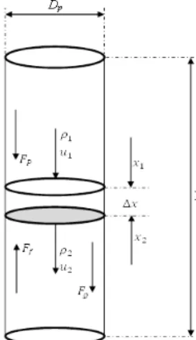
Fig. 2 shows a schematic flow diagram of an injection tube. A control volume of a section of the tube is considered for analysis and derivation of model governing equations. where
𝐹
𝑃,𝐹
𝑓,𝐹
𝑔,𝜌
and𝑢
are pressure force, frictional force, gravitational force, fluid density and velocity respectively. L, Dp and∆𝑥
are well depth, diameter and differential control volume.This study considers a purely vertical injection tube only hence, pipe inclination is unaccounted for. The following simplified assumptions are applied:
• One-dimensional flow in the pipe
• Homogeneous equilibrium fluid flow
• Negligible fluid structure interaction through vibrations
• Constant cross section area of pipe
The assumption of homogeneous equilibrium flow means that all phases are at mechanical and thermal equilibrium (i.e. phases are flowing with same velocity and temperature) hence the three conservation equations should be applied for the fluid mixture. Although, in practice usually the vapour phase travels faster than the liquid phase, the HEM model has been investigated proven to have an acceptable accuracy in many practical applications.
The mass, momentum, and energy conservation equations for a homogeneous two-phase flow model in a pipeline are rewritten in a differential form for numerical solution scheme [24]-[27] respectively as:
Mass conservation
𝜕𝜌𝑚
𝜕𝑡 + 𝜕𝜌𝑚𝑢𝑚
𝜕𝑥 = 0 (1)
Momentum conservation
𝜕𝜌𝑚𝑢𝑚
𝜕𝑡 + 𝜕
𝜕𝑥(𝜌𝑚𝑢𝑚2) + 𝜕𝑃 𝜕𝑥=
𝑓𝑤𝜌𝑚𝑢𝑚2
𝐷𝑝 − 𝜌𝑚𝑔 sin𝜃 (2)
Energy conservation
𝜕𝐸 𝜕𝑡+
𝜕𝑢𝑚(𝐸+𝑃)
𝜕𝑥 =
𝑓𝑤𝜌𝑚𝑢𝑚3
𝐷𝑝 − 𝜌𝑚𝑢𝑚𝑔 sin𝜃+
𝑄 𝜋𝑟
𝑤 2 (3) where
𝜌
𝑚,𝑢
𝑚, P,𝐷
𝑝,𝑟
𝑤, g,𝜃
is mixture density, mixture velocity, pressure, wellbore diameter, wellbore inner radius, wall friction coefficient, gravity and inclination angle of the wall respectively. The subscripts m and wdenote mixture and pipe wall.The wall friction between the fluid and pipe wall is described by the friction factor for pipes with rough walls
𝑓
𝑤, isdefined byChen’s correlation [28]:1
�𝑓𝑤=−2 log�
𝜀 𝐷⁄ 𝑝
3.7065− 5.0452
𝑅𝑒 log� 1 2.8257�
𝜀 𝐷𝑝�
1.1098 +
5.8506
𝑅𝑒0.8981�� (4) Q is the heat exchange between the fluid and its surrounding wall and formation.
𝑄=𝐷4
𝑒𝑞ℎ𝑓�𝑇𝑤− 𝑇𝑓� (5)
where the wellbore equivalent diameter is given as
𝐷
𝑒𝑞=
�
4𝐴𝜋 (6)E in (3) represents the total mixture energy defined as:
𝐸
=
𝜌
𝑚(
𝑒
+
12𝑢
𝑚2)
(7) The modified Peng-Robinson equation of state is given by [22] and [24] is applied using a reference data base REFPROP [29] incorporated with the model.III. NUMERICAL SOLUTION METHOD
In this study, an effective model based on the Finite Volume Method (FVM), incorporating a conservative Godunov type finite-difference scheme [30]-[32] is used. The FVM is well-established and thoroughly validated CFD technique. In essence, the methodology involves the integration of the fluid flow equations over the entire control volumes of the solution domain and then accurate calculation of the fluxes through the boundaries of the computed cells.
For the purpose of numerical solution of the governing equations they are written in a vector form [33]:
𝜕𝑄�⃗ 𝜕𝑡 +
𝜕𝑓⃗
𝜕𝑧=𝑆⃗, (8)
where
𝑄�⃗= (𝜌 , 𝜌𝑢 , 𝜌𝑒)𝑇,
𝑓⃗=�𝜌𝑢 , (𝜌𝑢2+𝑃) , 𝑢( 𝜌𝑢𝑒+𝜌𝑢2+𝑃)�𝑇
𝑆⃗= (𝑆𝑚, 𝑆𝑚𝑜𝑚, 𝑆𝑒)𝑇 (9) 𝑄�⃗, 𝑓⃗ and 𝑆⃗ are the vectors of conserved variables, fluxes and source terms respectively. The source terms 𝑆𝑚,
𝑆𝑚𝑜𝑚and
𝑆
𝑒 describe the effects of mass, momentum andheat exchange between the fluid and its surrounding respectively, as well as friction and heat exchange at the pipe wall.
The governing equations (9) form a set of quasi-linear hyperbolic equations, provided that they have distinct and real eigenvalues. Equations of such kind can be solved numerically using methods developed in computational gas dynamics [33], [34]. One of these methods is the finite volume method largely used for computation of transient compressible flows.
Applying the widely used and validated finite volume methodology, the spatial domain is discretised into a finite number of cells (control volumes or grid cells) and keeping track of an approximation of the integral of the flux over these volumes. In each time step the approximation of the flux through the endpoints of the interval is updated.
Denote the i-th grid cell by
𝐶𝑖=�𝑥𝑖−1/2,𝑥𝑖+1/2�, (10)
𝑄𝑖𝑛≈∆𝑥1 ∫𝑥𝑥𝑖−1/2𝑖+1/2𝑞(𝑥,𝑡𝑛)𝑑𝑥≡∆𝑥1 ∫ 𝑞𝐶𝐶𝑖𝑛 (𝑥,𝑡𝑛)𝑑𝑥 (11)
where ∆𝑥=𝑥𝑖+1/2− 𝑥𝑖−1/2 is the length of the cell.
Fig. 3. Cell variables and inter-cell fluxes in finite-volume discretisation of the special and time domains.
Then conservation equations are integrated over a control volume as can be seen in Fig. 3 to transform the differential equations to a finite set of algebraic equations. Integrating and rearranging (11) gives:
𝑄𝑖𝑛+1=𝑄𝑖𝑛−∆𝑡∆𝑥�𝐹𝑖+1
2
𝑛 − 𝐹
𝑖−𝑛12� (12)
where 𝐹𝑖−1𝑛 /2 is the approximation to the average flux along
∆𝑥=𝑥𝑖−1/2. Rewriting (12) becomes:
i n
i n i n i n
i S
x F F
t Q Q
= ∆
− +
∆
− + −
+
2 / 1 2 / 1 1
(13) where
Q
inis an average value for a piece wise constant with various subdomain in each cell for the i-th control volume, then
-th time step. Equation (13) uses explicit time integration scheme.A. Boundary Conditions
Setting appropriate boundary conditions at the top and bottom of the well is important given that in practice a finite set of grid cells are covering the computational domain. This means that, the first and last cells will not have the required neighbouring information on the left and right end respectively. In order to close the flow equations, relevant boundary conditions are added using a ghost cell at either end of the well.
Fig. 4. Schematic representation of the isenthalpic inflow condition in the ghost cell at the wellhead.
B. At the Top of the Well
C. At the Bottom of the Well
At the bottomhole, an empirical pressure-flow relationship derived from reservoir properties [20], [40] is employed:
𝐴̃+𝐵� ×𝑀+𝐶̃ × 𝑀2= 𝑃𝐵𝐻𝐹2 − 𝑃
𝑟𝑒𝑠2 (14)
where
𝐴̃ is the minimum pressure required for the flow to start
from the well into the reservoir,
𝐵� and 𝐶̃ are site-specific dimensional constants,
𝑀 is the instantaneous mass flow rate at the bottomhole,
𝑃𝐵𝐻𝐹2 is the instantaneous bottomhole pressure, and 𝑃𝑟𝑒𝑠2 is the reservoir static pressure.
Unlike [21] that used a standard linear relationship called “injectivity index” in describing the relationship between the reservoir and the bottom of the well. Equation (14) represents a more sophisticated condition than a standard, linear relationship between the bottomhole pressure and the flow rate given by an injectivity index.
IV. RESULTS
The model results obtained showed the impact of CO2
start-up injection operations on wellhead pressure and temperature, and the consequent flow of the CO2 stream
down the injection well. In a real CCS project however, the transient behaviour of CO2 during well start-up will be
observed based on the differences in wellbore depth, the injection flow rate, the injection pressure, the reservoir pressure, and the injection temperature. The start-up CO2
injection analysis is vital to predicting an optimum injection strategy for large-scale CO2 sequestration. The process of
injecting CO2 with higher pressure into a well with lower
pressure at the wellhead is similar to the expansion of a real gas which is released from a high pressure region to a low pressure region. Such process is characterised by an inevitable cooling of the gas upon entering the lower pressure domain and it is called the Joule-Thomson cooling effect.
The model input parameters were based on the Goldeneye CCS project injection well conditions are summarised in Table I [35]. Based on the simulation results obtained, the temperature, pressure and density profiles of CO2 in the
tubing at different depth and times are presented in Figures below.
TABLE I: GOLDENEYE INJECTION WELL AND CO2INLET CONDITIONS [35]
Input parameter Value
Wellhead pressure, bar 36.5
Wellhead temperature, K 280
Bottom-hole pressure, bar 82
Bottom-hole temperature, K 296
Well depth, m 2500
CO2 injection rate, kg/s 38
Injection tube diameter, m 0.125
CO2 inlet pressure, bar 50
CO2 inlet temperature, K 277
The wellhead pressure was maintained at 36.5 bar, and the wellhead temperature reached a thermal equilibrium with its surroundings at 7 oC. The hydrostatic pressure condition is the differential factor between the variations in wellhead pressure and bottom-hole pressure. It is likely that with relatively low reservoir pressure at an injection well, the wellhead pressure at start-up injection may be less than the corresponding saturation pressure at the ambient temperature. As a result of the lower pressure condition at the wellhead, more gaseous CO2 is present near the wellhead in the tubing
during well start-up injection. Fig. 4 shows a schematic representation of the isenthalpic
As can be seen in Fig. 5, the bottom-hole pressure gradually increased from the reservoir static pressure (82 bar) to about 110 bar after well start-up for 100 seconds. This means that the hole-bottom pressure increases with time as more CO2 is injected into the well resulting to a
corresponding increase in the wellhead pressure due to hydrostatic conditions.
0 500 1000 1500 2000 2500 0
20 40 60 80 100 120 140
P
res
s
ure (bar
)
Depth (m) Initial profile 100 s 300 s 500 s
Fig. 5. Wellbore pressure profiles of CO2 stream at different simulation
times.
As shown in Fig. 6, the temperature at the wellhead (at 0 m depth) dropped significantly within the first 100 sec due to the Joule-Thomson cooling effect of the expanding CO2.
Notably, there is a continuous decrease in temperature at the reservoir end from 296 K to 286, 282.5 and 281 K after 100, 300 and 500 sec respectively. This decrease can be attributed to the heat exchange between the surrounding formation and the incoming CO2 stream.
0 500 1000 1500 2000 2500
276 278 280 282 284 286 288 290 292 294 296 298
Tem
perat
ur
e (K
)
Depth (m) Initial profile 100 s 300 s 500 s
Fig. 6. Wellbore temperature profiles of CO2 stream at different simulation
times.
However, as CO2 pressure increases along the wellbore
(see Fig. 5 pressure profile) it tends to get colder and denser with such increasing pressure (see Fig. 6 temperature profile), as heat is lost to the surrounding formation and then the temperature drops as it approaches the reservoir end.
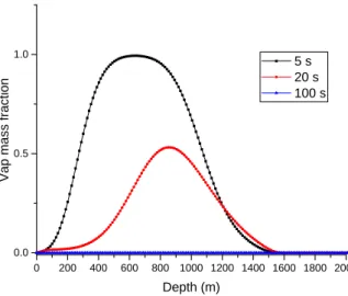
The density profile in Fig. 7 shows a clearer description of the CO2 stream behaviour going down the injection well. The
profiles of t after 5 and 20 seconds of simulation show a sudden decrease at about 400 m and later increases at about 1200 m down the injection well which likely corresponds to a possible phase transition. The CO2 density rises significantly
with well depth showing the presence highly dense CO2
stream composition down the well. Fig. 8 shows CO2 phase
diagram for density profile of various regions where the liquid region has higher densities followed by the supercritical region. At higher densities above 900 kg/m3 and temperatures above 273 K the CO2 stream is likely to be in
the supercritical or liquid phase.
0 500 1000 1500 2000 2500
0 200 400 600 800 1000
D
ens
it
y
(k
g/
m3)
Depth (m)
5 s 20 s 100 s
Fig. 7. Wellbore density profiles of CO2 stream at different simulation
times.
0 50 100 150 200 250 300 25
30 35 40 45 50 55 60 65 70 75 80 85 90 95 100 105 110
Pressure (800 m) Pressure (400 m) Pressure (Wellhead)
P
res
s
ure (bar
)
Time (s)
Fig. 9. CO2 stream pressure profiles at different well depths.
The pressure profile in Fig. 9 shows a sharp depressurisation at the start of injection due to the pressure difference between the incoming CO2 and the wellhead
pressure. The incoming CO2 (at 50 bar) expands upon
arriving at the wellhead with lower pressure (at 36.5 bar) attaining a record low pressure within the first 10 to 50
seconds. After which the pressure starts building up due to the hydrostatic condition and possible minimal frictional losses encountered by the fluid. The start-up injection test case at the wellhead showed a significantly low pressure was near 30 bar from the initial inlet pressure of 50 bar. The expanding gaseous CO2 at the wellhead and the
corresponding frictional losses along the wellbore greatly impacted on the pressure profile.
The temperature profile also follows a similar pattern like that of the pressure as can be seen in Fig. 10. However, greater temperature drop is predicted at the wellhead where the CO2 stream experienced a drastic expansion upon arriving
at a lower pressure region. Such expansion is accompanied by a significant temperature drop induced by Joule-Thomson cooling effect on an expanding gas as the dense-phase CO2
enters the injection well. Hence, the most significant cooling takes place at and near the wellhead during start-up operations compared with 400 and 800 m down the well. Notably, the results show a possibility of massive drop in temperature below the freezing point of water (i.e. 273 K) which poses serious safety concerns for large-scale CO2
sequestration projects. The presence of interstitial water molecules in the wellbore that come in contact with the injected CO2 may form hydrates or ice which could block the
injector inlet and cause severe operational challenges.
0 50 100 150 200 250 300 270
275 280 285 290 295 300 305
Tem
perat
ur
e (K
)
Time (s) Temp (800 m) Temp (400 m) Temp (Wellhead)
Fig. 10. CO2 stream temperature profiles at different well depths.
0 200 400 600 800 1000 1200 1400 1600 1800 2000 0.0
0.5 1.0
V
ap m
as
s
f
rac
ti
on
Depth (m)
5 s 20 s 100 s
Notably in Fig. 11, the vapour mass fraction over time shows CO2 expansion upon arriving at the wellhead indicated
by a rise in vapour mass fraction followed by a rapid drop as more fluid is injected. Such expansion is followed by rapid cooling which reduces the vapour composition quickly and this behaviour agrees with the previous observation of rapid temperature drop at the wellhead. The vapour fraction profile after 20 sec of simulation shows lower vapour composition in the CO2 stream compared with the profile after 5 sec of
simulation. However, it is noteworthy that the vapour mass fraction from wellhead to reservoir after 100 sec of simulation is constant at zero. This means that after 100 sec of simulation the CO2 stream pressure and temperature
reaches supercritical dense phase where the vapour phase totally disappears.
The simulation results of the current model show trends similar to those published in literature. Reference [20] used OLGA (OLGA 7 User manual, 2010) software for wellbore dynamics to predict the decrease in pressure and temperature of CO2 at the wellhead, as well as CO2 phase behaviour in the
wellbore during well transient operation.
As can be seen in Fig. 12, the wellhead pressure profile of the current simulation shows very similar trend with the profile obtained by [20]. Both results show an initial depressurisation from the inlet pressure (50 bar) to a value below the wellhead pressure (36.5 bar) before increasing due to continuous injection and hydrostatic pressure build-up from the bottom-hole.
0 50 100 150 200 250 300 28
32 36 40 44 48 52 56 60 64 68 72
P
res
sure (bar
)
Time (s)
Li et al, (2015 Current simul
Fig. 12. Comparison of CO2 stream wellhead pressure profiles.
Comparing the temperature profiles of the current simulation and [20], the trend is very similar as both predicted significant temperature drop. The gaseous CO2
expansion induced temperature drop at the wellhead due to Joule-Thomson cooling effect is observed in Fig. 13. Notably, [20] predicted much lower temperature drop (about 3 oC lower) than our current simulation result. This variation may be due to the different equation of state employed in predicting the thermodynamic properties of CO2. Reference
[20] used Span and Wagner equation of state to calculate the density and the specific heat of CO2, and
Soave-Redlich-Kwong [37] equation was used for calculating the viscosity and thermal conductivity of CO2. In
current model, we employed the Peng-Robinson equation of state to determine the phase equilibrium and all thermodynamic properties of CO2. Hence, the varying
equation of state used may therefore over-predict or under-predict some properties leading to high or low cooling
[20]
Current model
effect.
Fig. 13. Comparison of CO2 stream wellhead temperature profiles.
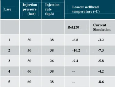
The model was further tested to establish an optimum start-up injection condition by alternating some parameters. The lowest wellhead temperature was monitored by varying the injection rate, injection pressure and injection temperature. As can be seen in Table II, the analysis showed the wellhead temperature is lower with decreasing injection rate and injection temperature but reverse is the case for injection pressure, which gives lower wellhead temperature when increased.
TABLE II: LOWEST WELLHEAD TEMPERATURE AT DIFFERENT INJECTION RATE AND INLET PRESSURE DURING START-UP
Case
Injection pressure (bar)
Injection rate (kg/s)
Lowest wellhead
temperature (◦C)
Ref.[20] Current
Simulation
1 50 38 -6.8 -3.2
2 50 38 -10.2 -7.3
3 50 26 -9.4 -5.8
4 60 38 -- -4.2
5 60 38 -- -8.6
V. CONCLUSIONS
This study identified very vital safety issues associated with CO2 sequestration in highly-depleted gas fields and
proffered possible ways of minimising the associated risk. The key safety issue was the possibility of large temperature drops at the wellhead which can induce thermal shocking on the steel casing leading to it fracture or can also form hydrates or ice with the interstitial water leading to injector blockage and eventual injection system failure.
As presented in the results session for the start-up injection case. Showing the possibility of large temperature drops at
the wellhead which poses serious safety challenges and requires proper approach and in other to minimise the threat it poses the following key points are noteworthy during start-up injection procedure:
• Rapid start-up injection is required to minimise temperature drop at the wellhead
• Higher injection flow rates will also help reduce the temperature drop during start-up injection.
• Minimal pressure difference between incoming CO2 and
wellhead pressure can minimise the Joule-Thomson cooling effect.
• Higher temperature for incoming CO2 can also minimise
the Joule-Thomson cooling effect.
• Increasing the injection pressure with time is required to avoid backflow and blowout situations, since there is continuous pressure build-up during injection.
REFERENCES
[1] IPCC, Climate Change 2014 Synthesis Report, Contribution of Working Groups I, II and III to the Fifth Assessment Report of the Intergovernmental Panel on Climate Change, pp. 1–151, 2014. [2] B. S. Fisher, N. Nakicenovic, K. Alfsen, J. C. Morlot, F. D. L.
Chesnaye, J.-C. Hourcade, and R. Warren, “Issues related to mitigation in the long-term context,” Climate Change 2007: Mitigation. Contribution of Working Group III to the Fourth Assessment Report of the Inter-Governmental Panel on Climate Change, pp. 196–250, 2007. [3] J. Blackford, S. Beaubien, E. Foekema, V. Gemeni, S. Gwosdz, D. Jones, and F. Ziogou, A Guide to Potential Impacts of Leakage from CO2 Storage, p. 61, 2010.
[4] United Nations, F. COP21 Agreement, 21930, December 2015. [5] COP21, “Paris Agreement, FCCC/CP/2015/L.9/Rev.1,” (PDF).
UNFCCC Secretariat.
[6] IEA, IEA Newsletter – June 2009, 2011.
[7] M. Lu and L. D. Connell, “The transient behaviour of CO2 flow with
phase transition in injection wells during geological storage – application to a case study,” Journal of Petroleum Science and
Engineering, vol. 124, pp. 7–18, 2014.
[8] M. Lu and L. D. Connell, “Transient, thermal wellbore flow of multispecies carbon dioxide mixtures with phase transition during geological storage,” International Journal of Multiphase Flow, vol. 63, pp. 82–92, 2014.
[9] A. Battistelli, P. Ceragioli, and M. Marcolini, “Injection of acid gas mixtures in sour oil reservoirs: Analysis of near-wellbore processes with coupled modelling of well and reservoir flow,” Transport in
Porous Media, vol. 90, no. 1, pp. 233–251, 2011.
[10] M. L. Michelsen, “The isothermal flash problem,” Part I & II. Stability,
Fluid Phase Equilibria, vol. 9, no. 1, pp. 1–19, 1982.
[11] E. Lindeberg, “Modelling pressure and temperature profile in a CO2
injection well,” Energy Procedia, vol. 4, pp. 3935–3941, 2011.
[12] Non-isothermal flow of carbon dioxide in
injection wells during geological storage,” International Journal of
Greenhouse Gas Control, vol. 2, no. 2, pp. 248–258, 2008
[13] K. Sasaki, T. Yasunami, and Y. Sugaia, “Prediction model of bottom hole temperature and pressure at deep injector for CO2 sequestration to
recover injection rate,” Energy Procedia, vol. 1, no. 1, pp. 2999–3006, 2009.
[14] B. Wiese, M. Nimtz, M. Klatt, and M. Kühn, “Sensitivities of injection rates for single well CO2 injection into saline aquifers,” Chemie Der
Erde - Geochemistry, vol. 70, pp. 165–172, 2010.
[15] J. Q. Shi, C. Imrie, C. Sinayuc, S. Durucan, A. Korre, and O. Eiken, Snøhvit CO2 storage project: Assessment of CO2 injection performance
through history matching of the injection well pressure over a 32-months period,” Energy Procedia, vol. 37, pp. 3267–3274, April 2008.
[16] J. Q. Shi, C. Sinayuc, S. Durucan, and A. Korre, “Assessment of carbon dioxide plume behaviour within the storage reservoir and the lower caprock around the KB-502 injection well at in Salah,” International
Journal of Greenhouse Gas Control, vol. 7, pp. 115–126, 2012.
[17] K. Michael, P. R. Neal, G. Allinson, J. Ennis-King, W. Hou, L. Paterson, and T. Aiken, “Injection strategies for large-scale CO2
storage sites,” Energy Procedia, vol. 4, pp. 4267–4274, 2011. [18] A. A. Afanasyev, “Multiphase compositional modelling of CO2
injection under subcritical conditions: The impact of dissolution and phase transitions between liquid and gaseous CO2 on reservoir
,
temperature,” International Journal of Greenhouse Gas Control, vol. 19, pp. 731–742, 2013.
[19] D. S. Hughes, “Carbon storage in depleted gas fields: Key challenges,”
Energy Procedia, vol. 1, no. 1, pp. 3007–3014, 2009.
[20] X. Li, R. Xu, L. Wei, and P. Jiang, “Modeling of wellbore dynamics of a CO2 injector during transient well shut-in and start-up operations,”
International Journal of Greenhouse Gas Control, vol. 42, pp. 602–
614, 2015.
[21] G. Linga and H. Lund, “A two-fluid model for vertical flow applied to CO2 injection wells,” International Journal of Greenhouse Gas
Control, vol. 51, pp. 71–80, 2016.
[22] R. Span and W. Wagner, “A new equation of state for carbon dioxide covering the fluid region from the triple-point temperature to 1100 K at pressures up to 800 MPa,” Journal of Physical and Chemical
Reference Data, vol. 25, no. 6, p. 1509, 1996.
[23] R. Stryjek and J. H. Vera, “PRSV: An improved Peng—Robinson equation of state for pure compounds and mixtures,” The Canadian
Journal of Chemical Engineering, vol. 64, no. 2, pp. 323–333, 1986.
[24] M. J. Zucrow and J. D. Hoffman, Gas Dynamics, vols. 1 and 2, Wiley, New York, 1976.
[25] H. Mahgerefteh, P. Saha, and I. G. Economou, “Fast numerical simulation for full-bore rupture of pressurized pipelines,” A.I.Ch.E. Journal, vol. 45, no. 6, p. 1191, 1999.
[26] S. Brown, J. Beck, H. Mahgerefteh, and E. S. Fraga, “Global sensitivity analysis of the impact of impurities on CO2 pipeline failure,”
Reliability Engineering and System Safety vol. 115 pp. 43 54 2013
[27]
[28] L. Cheng, G. Ribatski, L. Wojtan, and J. R. Thome, “New flow boiling heat transfer model and flow pattern map for carbon dioxide evaporating inside tubes,” Int. J. Heat Mass Transfer, vol. 49, pp. 4082–4094, 2006.
[29] E. W. Lemmon, M. O. McLinden, and D. G. Friend. (2010). Thermo- physical properties of fluid systems, in NIST Standard Reference Database 69. Natl. Inst. of Stand. and Technol., Gaithersburg, Md. [Online]. Available: http://webbook.nist.gov
[30] S. K. Godunov. “A difference scheme for numerical solution of discontinuous solution of hydrodynamic equations,” Mat. Sbornik, vol. 47, pp. 271-306, 1969.
[31] Y. G. Radvogin, Y. B. Rykov, and N. A. Zaitsev, “Computation of non-stationary swirled flows in nozzles and pipes using new 'explicit-implicit' type scheme,” Rep. KIAM Preprint № 52, vol. 58, 2011.
[32] P. S. Cumber, M. Fairweather, S. A. E. G. Falle, and J. R. Giddings “Predictions of the structure of turbulent, moderately underexpanded jets,” Journal of Fluids Engineering-Transactions of theAsme, vol. 116, no. 4, pp. 707-713, 1994.
[33] E. Toro, The HLLC Riemann Solver Abstract : This Lecture is about a
Method to Solve Approximately, 2012.
[34] R. J. LeVeque, “Finite volume methods for hyperbolic problems,”
Cambridge University Press, vol. 54, p. 258, 2002.
[35] T. R. Shell UK. (2015). Peterhead CCS Project. [Online]. Available: https://www.gov.uk/government/news/peterhead-carbon-capture-and-storage-project
[36] Q. Zhao and Y.-X. Li, “The influence of impurities on the transportation safety of an anthropogenic CO2 pipeline,” Process
Safety and Environmental Protection, vol. 92, no. 1, pp. 80–92, 2014.
[37] L. Paterson, M. Lu, L. Connell, and J. P. Ennis-King, “Numerical modeling of pressure and temperature profiles including phase transitions in carbon dioxide wells,” Society of Petroleum Engineers, 2008.
[38] K. W. Thompson, “Time dependent boundary conditions for hyperbolic systems,” J. Comput. Phys., vol. 68, no. 1, pp. 1–24, 1987. [39] K. W. Thompson, “Time-dependent boundary conditions for
hyperbolic systems, {II},” J. Comput. Phys., vol. 89, pp. 439–461, 1990.
[40] Shell, Peterhead CCS Project, 2015.
Revelation J. Samuel was born in Nembe, Bayelsa State, Nigeria on May 27, 1985. Mr Samuel obtained an outstanding first degree (B.Eng) in chemical engineering from Niger Delta University, Nigeria in 2009 and M.Sc. in chemical process engineering from UCL in 2013 after securing a fully funded scholarship award in 2012 from Shell Nigeria. He joined UCL Chemical Engineering Department in 2015 as a postgraduate researcher after securing a fully funded scholarship award in 2014 from Petroleum Technology Development Fund, Nigeria.
His main research areas include multiphase flow modelling, pipeline safety and risk management and Carbon Capture and Sequestration (CCS) supervised by Prof. Haroun Mahgerefteh.
Mr Samuel is a member of the Institute of Chemical Engineers (IChemE) and has over ten publications in various journals.
Haroun Mahgerefteh obtained his PhD in chemical engineering from Imperial College London. His main research expertise are in multi-phase CFD flow modelling of hydrocarbon transportation pipelines, safety and loss prevention in the oil and gas industries, particularly with reference to pipeline rupture safety assessment where he supervises several chemical engineering students for PhD studies.
His main research expertise is in safety and loss prevention in the oil and gas industries, particularly modelling highly transient multi-phase flows following pipeline rupture. He is the coordinator of European Commission FP7 projects, CO2PipeHaz and CO2QUEST
involving collaboration between 18 academic institutions and industry partners across Europe, Canada and China as well as co-investigator in EPSRC MATTRAN and National Grid COOLTRANS projects.
Prof Mahgerefteh is the graduate admissions tutor and programme manager for our highly successful MSc programme in chemical process engineering, a chartered engineer, fellow of the institution of chemical engineers, and member of the IChemE Subject Group in safety and loss prevention. He has over a hundred publications in various international journals.
, , , .
M. M. Arzanfudi and R. Al-khoury, A Compressible Two-Fluid
Multiphase Model for CO2Leakage through a Wellbore, pp. 477–507,