Abstract—In this paper, the most widely used
empirical path loss models are compared to real data; the most appropriate one (COST-231) has been optimized using three different algorithms to fit measured data for mobile communication system. The performance of the adjusted Cost-231 model obtained by the proposed methods is then compared to the experimental data. The concert criteria selected for the comparison of various empirical path loss models is the Root Mean Square Error (RMSE). From numerical simulations, it was noticed a significant improvement in the prediction made by the proposed algorithm with a slight superiority of Invasive weed Optimization algorithm in term of lower RMSE value in one hand and in term of convergence speed on the
other hand compared to PSO and ABC algorithm.
Index Terms— Empirical models, Mobil communication, Path Loss, COST-231, Invasive weed Optimization.
I. INTRODUCTION
The need for connectivity anywhere, added to the increment in the number of users, has caused the development of various generations of mobile communication standards in the last decades. The demand for greater traffic capacity involving both voice and data transmission requires the planning of mobile communication networks comprised of smaller and smaller cells, thus making the number of base stations grow exponentially, and complicating the process of optimizing the location of these stations. Because of this, accurate prediction models are needed for making received signal level/path loss predictions prior to actual network deployment.
In telecommunication industry, path loss is the reduction in power density of an electromagnetic wave signal as it propagates from the transmitter to the receiver [1].
Houcine Oudira: University of Mohamed Boudiaf Laboratory of electrical engineering M’Sila, Algeria houcine.oudira@univ-msila .dz
Lotfi Djouane: University of Mustafa ben boulaid, Batna2 Laboratory of electrical engineering M’Sila, Algeria [email protected]
Messaoud Garah: University of Mohamed Boudiaf Laboratory of electrical engineering M’Sila, Algeria [email protected]
During the planning stage of cellular networks, models are employed to predict the behavioral characteristics of signals using similar attributes and constraints of the environment before deployment. Traditional path-loss prediction model mainly used experimental models such as Egli 1, SUI models, which briefly be introduced in the section 2. The problem of these models is that expressions are based on the qualitative propagation environments such as urban, suburban and open areas. However, in practice, empirical path loss model tuning is usually required due to significant drop in prediction performance of empirical models when applied in the environments other than the ones they are designed.
In the last few years, many researchers have applied different algorithms to predict the path loss in theirs environments [2-6]. To this effect, we need to optimize empirical models to provide optimal parameters for radio-wave path-loss prediction in the target area and have good cellular palanification [7-9].
In this paper, we analyze the performance achievable with intermediate techniques, between purely empirical models and real measure established from the field of study, based on the use of Invasive weed Optimization, particle swarm optimization and artificial bee colony algorithm. First of all the most widely used empirical path loss models: «Cost-231», «Hata», «SUI» and «Egli» are compared to real data; the most appropriate one is then optimized. This technique is employed to curb the problem observed in the differences between the used empirical models and the actual measured data in a particular environment [10].
This latter is the main issue discussed in this paper in which, the performance of the adjusted Cost-231 model obtained by the proposed methods is then compared to the experimental data. The concert criteria selected for the comparison of various empirical path loss models is the Root Mean Square Error (RMSE). From numerical simulations, it was noticed a significant improvement in the prediction made by the proposed algorithm with a slight superiority of IWO algorithm in term of lower RMSE value in one hand and in term of convergence speed on the other hand compared to PSO and ABC method and
Optimization of Suitable Propagation Model for
Mobile Communication in Different Area
to the genetic algorithm and Nelder-Mead method proposed in [5] and [6] respectively.
The rest of this paper is organized as follows. In section 2 we review the empirical models and the proposed algorithms. Methodology and application are presented in section3. In section 4 presents the results and discussion. Finally, our conclusion and potential future work are presented in section5.
II. DATAOFPROBLEMTOBESOLVED
A. Optimization Algorithm
In this paper, to solve the path loss problem, the Invasive weed Optimization, particle swarm optimization algorithm and the artificial bee colony method are considered to minimize the difference between the used empirical models and the actual measured data.
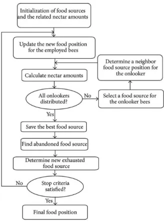
1) Artificial bees colony Algorithm ABC algorithm is a heuristic optimization algorithm introduced by Karaboga (Karaboga, 2005) inspired from how honey bees work together for collecting nectar from flowers. In ABC, the objective is to find the patch of flowers with maximum nectar amount (optimal solution). For achieving this, the bees are subdivided into three categories such as employed, onlooker and scout bees. Each one represents a D-dimensional solution, the bee which finds the best food source among all is most likely to be followed by other bees for converging to the best location. The aim of employed bees is to exploit the nectar sources explored before and share the information with the waiting bees (onlooker bees) in the hive. This information are related to the quality of food source sites exploited by the employed bees, based on this information, the onlooker bees inside the hive decide on the food source to exploit. The goal of the scout bees is to search randomly around the hive in order to find a new food source site [8]. In ABC algorithm the number of employed bee and onlooker bee is equal to the number of solutions in the population. The artificial bee colony algorithm consists of four main phases. Initial phase, employed bee phase, onlooker bee phase and scout bee phase.
To sum up, the ABC utilizes the concept of memory for storing personal best location. A bee visits randomly a new location and later it compares with the best location that it visited previously. If the new location is better, the old one is forgotten and the new location is memorized; otherwise, the memory remains unchanged. The basic steps of the
ABC algorithm are summarized and depicted via flowchart given in Fig. 1 [11-12]:
Fig. 1: ABC algorithm flowchart
2) Particle Swarm Optimization
The Particle swarm optimization is a population-based algorithm for searching global optimization problems introduced by Kennedy and Eberhart in 1995 [13]. It has the capability to find global optimal points by using the social interaction of unsophisticated agents. PSO utilizes a population (called swarm) of particles in the search space. The status of each particle is characterized according to its position and velocity.
𝑥𝑖
⃗⃗⃗ = (𝑥𝑖1, 𝑥𝑖2, 𝑥𝑖3, … . , 𝑥𝑖𝑑 )
and
𝑣𝑖
⃗⃗⃗ = (𝑣𝑖1, 𝑣𝑖2, 𝑣𝑖3, … . , 𝑣𝑖𝑑 ).
To discover the optimal solution, each particle changes its searching direction according to two factors: the best position of a given particle 𝑥𝑙𝑖 and
the best position (global pest) 𝑥𝑔 of the entire
swarm. PSO searches for the optimal solution by updating the velocity and position of each particle according to the following equations:
𝑥𝑖(𝑡 + 1) = 𝑥𝑖(𝑡) + 𝑣𝑖(𝑡 + 1) (1)
The velocity updates are calculated as a linear combination of position and velocity vectors
𝑣𝑖(𝑡 + 1) = 𝑤𝑣𝑖(𝑡) + 𝐶1𝜌1(𝑥𝑙𝑖(𝑡) − 𝑥𝑖(𝑡)) +
Where t denotes the iteration in the evolutionary space. w is the inertia weight. 𝐶1 and 𝐶2 are
personal and social learning factors. 𝜌1 and 𝜌2 are
random values uniformly distributed within the range [0, 1].
The basic process of the PSO algorithmis carried out with four basic operations: initialization, constraint handling, actualization, evaluation and selection [13]. Figure 2 shows its flowchart.
Fig. 2: PSO algorithm flowchart
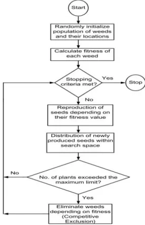
3) The Invasive weed Optimization
The Invasive weed Optimization is a stochastic optimization algorithm which inspired from weed colonization. Weeds have shown to be very robust and can quickly adapt to any environment. Thus, capturing their properties lead to a powerful optimization algorithm [14]. Some of the distinctive properties of IWO in comparison with other evolutionary algorithms are the way of reproduction, spatial dispersal, and competitive exclusion [15].
Considering an N variable optimization problem, the IWO process begins with initializing a population. That is, a population of initial solutions is randomly generated over the solution space. In optimization problems, seeds and field represent randomly generated initial solutions and N dimensional problem space, respectively. The fitness of each seed is calculated based on a predefined objective function of the problem. In other words, the number of seeds for each member varies linearly between Smin for the worst member
and S max for the best member. In the next step for implementing IWO, These seeds are then randomly scattered over the search space by normally distributed random numbers with mean equal to zero and varying standard deviation. The standard deviation is started from a predefined initial value (σinitial) and reduced to a final value (σfinal) and calculated based on
σiter= (1 − (iter iter max
⁄ ))n(σinitial− σfinal)
+ σfinal
(3) where itermax is the maximum number of
iterations, σiter is the SD at the current iteration and
n is the nonlinear modulation index. The produced seeds, accompanied by their parents are considered as the potential solutions for the next generation.
Once all seeds found their positions and the new plants grew to the flowering plants, they are ranked together with their parents. Some of the existing plants are then removed based on a competitive exclusion process, and an elimination mechanism is adopted such that plants with better ranking have more chance to survive.
This process is continued until the convergence criteria are met. A flow chart describing the IWO algorithm is presented in Fig. 3
B. Path loss Models
In wireless channels, the path loss prediction is very important factor that enables planning the effective transmitted power, coverage area and quality of service. However, several global and local parameters will affect path-loss prediction model. Empirical models describe from a statistical point of view the relationship between the path loss and the environment. Results are usually obtained by means of measurement campaigns.
In this paper, we have considered four various Empirical models for our study as follows:
1) Egli Model
Egli prediction model is an empirical model which has been proposed by [16]. Based on real data the path-loss approaching can be formulated as following:
𝑃𝐿 = 20 log(𝑓𝑐) + 40 log(𝑑) − 20 log(ℎ𝑡𝑒) +
{76.3 − 10 log(ℎ𝑟𝑒) , ℎ𝑟𝑒≤ 10𝑚 85.9 − 20 log(ℎ𝑟𝑒) , ℎ𝑟𝑒≥ 10𝑚
(4)
where
ℎ
𝑡𝑒= height of the base station antenna (m).ℎ
𝑟𝑒= height of the mobile station antenna (m).𝑑
= distance from base station antenna (km). f = frequency of transmission (MHz).2) Okumura Hata Model
Basically, this model has been introduced to urban areas; and with some correction factors it could be extended to suburban and rural areas. For urban area the median path loss equation is given by
PL(urb)(dB) = 69.55 + 26.16log(fc) − 13.82 log(hre) − a(hre) + (44.9 −
log(hte))log d (5)
For suburban area, it is expressed as
PL(suburban)(dB) =
PL(urban) − 2[log(fc/28)]2 − 5.4 (6) Finally, for open rural area, it is modified as
PL(open)(dB) = PL(urban) − 4.78(log(fc))2 + 18.33 log(fc) − 40.94 (7) The correction factor, (a(hre)), in Equation (5),
differs as a function of the size of the coverage area. For small and medium areas, it is
a(hre) = (1.1log(fc) − 0.7)hre− (1.56logfc −
0.8)dB (8) For large area, it is
a(hre) = 8.29(log1.54hre)2 − 1.1dB
for fc < 300𝑀𝐻𝑧 (9a)
a(hre) = 3.2(log11.75hre)2 − 4.97dB
for fc > 300MHz (9b) In the above equations, d is the transmitter-receiver antenna separation distance and it is valid for this range 1km–20km, fc represents the operating frequency from150 MHz to 1500 MHz.
The transmit antenna height, hre, ranges from 30m
to 200m and the receive antenna height, hre, ranges
from 1m to 10m are considered [17,18]. 3) Cost 231 Hata Model
The COST 231 model, sometimes called the Hata model PCS extension, is an improved version of the Hata model. It is widely used for predicting path loss in mobile wireless system.
It is designed to be used in the frequency band from 1500 MHz to 2000 MHz. It also includes corrections for urban, suburban and rural (flat) environments [19][20].
PL(d)(dB) = 46.3 + 33.9 log(fc) −
13.82 log(hte) − a(hre) + (44.9 −
6.55 log(hte)) log(d) + CM (10)
Where CM is a corrective term, CM=0 dB for
medium sized city and suburban area with moderate tree city or CM =3 dB for metropolitan centers.
Validity range of this model is:
1500 MHz < 𝑓 < 2000 𝑀𝐻𝑧, 30 m < hte< 200 𝑚,
1 m < hre< 10 𝑚, 1 km < 𝑑 < 20 𝑘𝑚.
4) SUI Model
The IEEE 802.16 wireless network standards consortium group proposed some standards for the frequency range below 11 GHz, having the channel model developed by Stanford University, or SUI model. This model takes the legacy of Hata model’s frequency extension for more than 1800 MHz. Little bit of correction in parameters, can be extended up to 3 GHz band frequency.
In this model, the BS antenna height can be varied from 10 m to 80 m and receiver end the height can vary between 2 m to 20m [21]-[22]. Innovation of this model is the introduction of the path loss exponent ɣ, and the weak fading standard deviation, S, as random variables obtained through a statistical procedure. The value of standard deviation of S is typically 8.2 to 10.6 dB [23].
SUI model comes out with three different types of terrain like terrain A dense urban locality, terrain B has hilly regions and terrain C for rural with moderate vegetation. The general path loss expression according to the SUI model is given by [24]
PL(db) = A + 10γlog10( d
d0) + Xf + Xh + s (11) where d > d0 (d in meters) is the distance between
the base station and the receiving antenna,
d0=100m, Xf is a correction for frequency above
2GHz, Xh is a correction for the receiver antenna
height, and s is a correction for shadowing because of trees and other clutters on a propagation path.
Parameter is defined as follows
A = 20log (
4πd0where is the wavelength in meters. Path loss exponent given by [25]
γ= a − b. hte+ c h te
⁄ (13) where hteis the base station antenna height in
meters, and a, b and c are constants dependent on the terrain type, as given in Table 1.
The correction factors for the operating frequency and for the receiver antenna height for the model are
X f= 6.0 log ( fc
2000) (14)
and, for terrain type A and B;
Xh = −10.8 log ( hre
2000); (15)
For terrain type C;
Xh= −20 log ( hre
2000) (16)
Where f, is the frequency in MHz, and ℎ𝑟𝑒 is the
receiver antenna height in meters. The SUI model is used for path loss prediction in rural, suburban and urban environments.
TABLE1. MODEL PARAMETERS FOR DIFFERENT TERRAINS
Model Parameter
Terrain A Terrain B Terrain C
a b (m-1) c (m)
4.6 0.0075 12.6
4.0 0.0065 17.5
3.6 0.005 20
III. EXPERIMENTALSETUP
The Batna city (Algeria) was selected to obtain the measurements. The drive test experimental was made in a radius of 1 km for BTS1 covering a small rural area crossing a road in the village 6 km from the city center of Batna, alongside BTS2 covering the area with a radius of 2.5 km, the propagation medium around this region is classified as a suburban area, it is assumed that an automatic handover occurs to adjacent base stations, when the signal strength is low. The emission sites specifications of these bases and their positions are shown in Table 2.
Data were collected when driving a car, having the experimental configuration. It consists of a Special Mobile Phone (Huawei U6100) GPS receiver (NMEA), a receiving antenna, and a laptop with a key and a drive test software (Huawei GENEX Probe). The vehicle was driven within the base station coverage area while continuously recording the received signal. Fig.4 and 5 show the measured signal strength and coverage of GSM network for the two BTS respectively. At every moment of the collected measurements, GPS data is also recorded simultaneously.
The information of the base station such as the frequency of transmission or reception, transmitted
power and antenna heights are obtained from the operator "Mobilis" of the Batna city for analysis. With the help of GPS data, and the location of base stations, the radial distances from the base station at any point along the route can be calculated.
TABLE 2. BTS PARAMETERS
Parameters BTS1 BTS2
Region type Rural Suburbain
Transmit power (dBm) 46 43
Cable Loss + Body loss 10.5 9.7
Transmitting antenna gain (dBi) 17.5 16.7
Receive antenna gain (dBi) 0 0
Transmit antenna height (m) 25 35
Mobile station antenna height (m) 1.5 1.5
Operating frequencies (MHz)
Uplink frequency
908 912,4
Downlink frequency
953 957,4
Geographic coordinates (°)
Latitude 35,2524 °N 35,62437 °N Longitude 6,13074 °E 6,36984 °E
Fig.4. Reception quality and coverage for BTS1
IV. RESULTSANDDISCUSSION A. Comparison with Prediction Models To investigate the prediction process, a comparison between predicted and measured path loss models have been performed for two base stations BTS1 and BTS2. The values of the predicted and the measured path loss are plotted against the separation distance between the Base Station (BS) antenna and the Mobile Station (MS) antenna (Figures 6 and 7). The values of Root Mean Square Error (RMSE), that are used to measure the forecasting accuracy of these models, are tabulated in Table 3.
TABLE 3. PERFORMANCE COMPARISON BETWEEN USED MODELS ACCORDING TO THE TEST CRITERIA
From Table 3, it is found that the performance of the COST 231 Hata model is the best one as the RMSE is the lowest value compared to other models. Figure 6 and 7 consolidate the result that COST 231 Hata model is the closest one to the measured path loss. Based on this observation, the COST 231 Hata model is selected as the best model for optimization process to develop a new model for the path loss prediction in Batna city for GSM 900 system.
Fig.6. Comparison between predicted and measured path loss for BTS1
Fig.7. Comparison between predicted and measured path loss for BTS2.
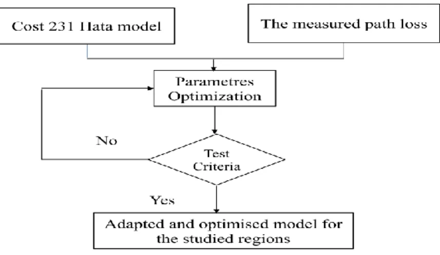
B. Optimization Process
In this study, the problem to be solved is formulated as a single mathematical equation that has five variables. Equation (17) must be defined in a manner make it a suitable model with actual field measurements, assessed by a cost function to a stopping criteria depends on the desired performance (Figure 8). This cost function is generally defined as the RMSE (Root Mean Square Error).
COST 231 Hata (rural/sub) model is defined as
𝑃𝐿 = 46.3 + 44.9 log(𝑑) − 13.82 log(ℎ𝑡𝑒) −
6.55 log(ℎ𝑡𝑒) log(𝑑) + 33.9 log(𝑓𝑐) − 𝑎(ℎ𝑟𝑒) (17)
The fitness function thatis used for the evaluation and parameters adjustment is defined by the mean square error (RMSE) as:
𝑅𝑀𝑆𝐸 = √∑𝑛𝑖=1|𝑃𝐿𝑚,𝑖−𝑃𝐿,𝑖|²
𝑛 (18)
Where 𝑃𝐿𝑚 represents the measured path loss in
dB, 𝑃𝐿 is the predicted path loss in dB, and 𝑛 is the number of the measured data points.
Path loss model optimization is a process in which a theoretical propagation model is adjusted with the help of measured values obtained from test field data. The aim is to get the predicted field strength as close as possible to the measured field strength.
0 0.1 0.2 0.3 0.4 0.5 0.6 0.7
20 40 60 80 100 120 140 160 180
Distance (Km)
P
a
th
L
o
s
s
(
d
b
)
Empirical Models In Rural Area
Cost231 Hata Rural measured data SUI type C Egli
0 0.5 1 1.5 2 2.5
20 40 60 80 100 120 140
Distance (Km)
P
a
th
L
o
s
s
(
d
b
)
Cost231 Hata Sub measured data SUI type B Egli
Base station
Cost-231
Hatas Sui
(c/b)
Fig 8. Flow chart of the optimization process
C. Optimization results
Simulation results are presented in the following tables and figures in which table 4 and 5 show predicted path loss values for existing models, measured data and optimized data of the BTS1 and BTS2 respectively . Fig 9 illustrated a comparative plot of optimized models, Cost 231 model and measured data for the BTS1 while Fig. 10 showed a plot comparing the optimized models with Cost 231 model and measured data for the BTS2.
TABLE 4: PATH LOSS VALUES FOR EXISTING MODELS, MEASURED AND OPTIMIZED MODEL OF BTS1
Distance
(km) SUI C Model
(dB)
Okumura Hata Model
(dB)
Egli Model (dB)
Cost 231 Model (dB)
Measured (dB)
Optimized Model
(dB)
0.112 85.2949 147.2408 68.1309 93.9246 118 125.685
0.2 96.0598 156.2414 78.2033 102.9253 134 130.743
0.302 103.7111 162.6387 85.3624 109.3225 138 134.309
0.4 108.9288 167.0013 90.2445 113.6851 139 136.790
0.5 113.0718 170.4652 94.1209 117.1491 141 138.7372
TABLE 5: PATH LOSS VALUES FOR EXISTING MODELS, MEASURED AND OPTIMIZED MODEL OF BTS2
Distance
(km) SUI b Model
(dB)
Okumura Hata Model
(dB)
Egli Model (dB)
Cost 231 Model (dB)
Measured (dB)
Optimized Model
(dB)
0.2 74.6843 86.4236 74.7434 101.1075 123.863 127.411
0.4 80.3382 92.8947 87.4848 112.1818 132.884 128.834
0.6 87.4768 98.7068 94.1680 118.0002 128.868 129.548
0.8 93.2477 103.4054 99.5708 122.6989 130.738 130.104
1 97.1927 106.6175 103.2643 125.9109 129.759 130.616
1.2 100.4787 109.2929 106.3406 128.5863 132.863 130.976
1.4 103.4559 111.7169 109.1280 131.0103 134.859 1.31.130
1.6 105.9006 113.7073 111.4168 133.0008 131.792 131.330
1.8 108.1426 115.5332 113.5163 134.8267 130.814 131.585
2 110.1668 117.1809 115.4109 136.4743 131.766 131.825
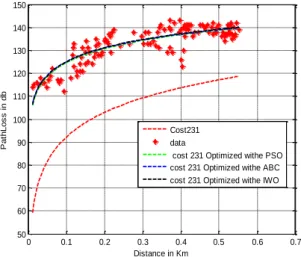
Fig 9. Comparison between COST-231 and optimized models (BTS1).
Fig. 10. Comparison between COST-231 and optimized models (BTS2).
TABLE 6. PERFORMANCE COMPARISON BETWEEN MEASURED AND TUNED MODELS ACCORDING TO THE TEST CRITERIA
(RMSE). Base station Cost 213 Cost IWO Cost ABC Cost PSO Cost GA (Test 03) [5] Cost N-M [6] BTS1 27.2553 4.142 4.1514 4.1427 5.4327 4.1614
BTS2 14.4196 3.038 3.0681 3.0493 3.0682 3.1681
From the optimization process of Cost 231 model, the developed models demonstrated better prediction compared to the existing models in terms of overall performance as shown in table 6. This remark is highlighted by the figures 9 and 10.
A closer look at table 6 turns out that the IWO method provides the lowest RMSE values in the two cases compared to the other proposed methods in one hand and to genetic algorithm and Nelder-Mead optimization proposed in [5] and [6] on the other hand.
The convergence speed of these methods during the optimization process is represented in figure (11), the IWO algorithm can converge rapidly compared to the other competitors.
Fig 11. Fitness function evolution versus number of iterations
V. CONCLUSION
Three optimization algorithms were proposed and tested in this paper to tune the parameters of Cost 231 Hata Model. Because, there is a need for considering the topology factor in propagation prediction models to achieve optimum design, the tuning models were verified by comparison with the measurements collected by the test driver technique in the rural and suburban environments in Batna city. The comparison results show a high degree of reduction in the path loss prediction. The slight superior performance of the IWO algorithm can be ascribed to two causes. First, The IWO can converge rapidly than the other proposed methods. Second, the IWO model can provide optimal parameters for radio-wave path-loss predicting with the smallest RMSE. Also a comparison with reference [5] and [6] confirms the same remarks obtained before. From the numerical results, it is obvious that adjusted COST 231 Hata model shows the closest agreement with the measurement result. Hence COST 231 Hata model with proposed modification is a good candidate for rural and suburban area of Batna.
For future work, forecasting other environments (Urban area) of path-loss data, taking in consideration the atmospheric factor, by using more powerful algorithm for propagation prediction models, to achieve optimum design of next
0 0.1 0.2 0.3 0.4 0.5 0.6 0.7
50 60 70 80 90 100 110 120 130 140 150
Distance in Km
P a th L o s s i n d b Cost231 data
cost 231 Optimized withe PSO cost 231 Optimized withe ABC cost 231 Optimized withe IWO
0 0.5 1 1.5 2 2.5
70 80 90 100 110 120 130 140
Distance in Km
P a th L o s s i n d b Cost231 data
cost 231 Optimized withe ABC cost 231 Optimized withe PSO cost 231 Optimized withe IWO
0 100 200 300 400 500 600 700 800 900 1000 100 101 102 Iteration B e s t C o s t
generation communication systems is a challenging issue for study.
REFERENCES
[1] C. S. Hanchinal, K. N. Muralidhara “A Survey on the Atmospheric Effects on Radio Pathloss in Cellular Mobile Communication System”. IJCST vo l. no.7, pp. 120-124, 2016.
[2] N.T. Surajudeen Bakinde, N. Faruk, A.A. Ayeni, M.Y. Muhammad, M.I. Gumel, “Comparison of Propagation Models for GSM 1800 and WCDMA Systems in Selected Urban Areas of Nigeria”. International Journal of Applied Information Systems (IJAIS), vol. 2, no.7, pp. 6-13, 2012. [3] C.O. Julie, M.U Onuu, J.O. Ushie, B.E. Usibe,
“Propagation Models for GSM 900 and 1800 MHz for Port Harcourt and Enugu, Nigeria”. Network and Communication Technologies, vol. 2, no.2, 2013. [4] J. Isabona, C.C. Konyeha, “Urban Area Path loss
Propagation Prediction and Optimization Using Hata Model at 800MHz”. IOSR Journal of Applied Physics (IOSR-JAP), vol. 3, pp. 8-18, 2013.
[5] M.Garah et al, "Path Loss Models Optimization for Mobile Communication in Different Areas", Indonesian Journal of Electrical Engineering and Computer Science, vol.3, pp.126-135, 2016.
[6] L. Djouane, H. Oudira “Empirical Model Optimization Using NelderMead Algorithm for Mobile Communication in Suburban and Rural Area” 3rd International Conference on Electrical and Information Technologies ICEIT’, 978-1-5386-1516-4/17/$31.00 © IEEE, 2017
[7] I. Israr, M. Shakir, M.A. Khan, S.A. Malik, S.A. Khan. “Path Loss Modeling of WLAN and WiMAX Systems” International Journal of Electrical and Computer Engineering (IJECE), vol. 5, no.5, pp. 1083-1091, October 2015.
[8] J.O. Famoriji, Y.O. Olasoji “Radio Frequency Propagation Mechanisms and Empirical Models for Hilly Areas” International Journal of Electrical and Computer Engineering (IJECE) vol. 3, no.3 , pp. 372-376. June 2013.
[9] V.H. Hinojosa, R. Araya “Modeling a mixed-integer-binary small-population evolutionary particle swarm algorithm for solving the optimal power flow problem in electric power systems” Applied Soft Computing, vol.13, pp3839–3852. 2013.
[10] Diawuo k, Dotche K.A and Toby Cumberbatch, “Data fitting to Propagation Model using Least Square Algorithm: A case of Ghana”, International Journal of Engineering Sciences, vol. 2, no.6, pp. 226 -230, June 2013.
[11] D. Karaboga, "An idea based on honey bee swarm for numerical optimization," Technical report-tr06, Erciyes university, engineering faculty, computer engineering department 2005.
[12] W. Gao, S. Liu, and L. Huang, "A global best artificial bee colony algorithm for global optimization," Journal of Computational and Applied Mathematics, vol. 236, pp. 2741-2753, 2012.
[13] R. Eberhart, J. Kennedy, “ A New Optimizer Using Particle Swarm Theory”, Sixth International Symposium on Micro Machine and Human Science 0-7803-2676-8/95 $4.00 0 IEEE, 1995
[14] AR. Mehrabian, C. Lucas, “A novel numerical optimization algorithm inspired from weed colonization”, Ecological Informatics, vol. 1, no.4, pp. 355–366. 2006. [15] A. Ashik , A.B.M. Ruhul “Performance Comparison of
Invasive Weed Optimization and Particle Swarm Optimization Algorithm for the tuning of Power System Stabilizer in Multi-machine Power System”, International Journal of Computer Applications, vol. 41, no.16, pp. 29-36, 2012.
[16] J. J. Egli, “Radio propagation above 40 Mc over irregular terrain”, Proc. IRE, vol. 45, no. 10, pp. 1383–1391, 1957. [17] T. K. Sarkar, T. K., Z. Ji, K. J. Kim, A. Medour, M.
SalazarPalma, “A survey of various propagation models for mobile communication,” IEEE Antennas and Propagation Magazine, vol. 45, no.3, pp. 51–82, Jun. 2003
[18] M. Hata, “Empirical formula for propagation loss in land mobile radio services”, IEEE Trans. Veh. Technol., vol. vt-29, no.3, pp. 317-325, Agt. 1980.
[19] J. D. Parsons, “The Mobile Radio Propagation Channel”, 2nd ed.,Wiley,West Sussex, 2000.
[20] T. Asztalos. “Planning a WiMAX Radio Network with A9155”. Alcatel-Lucent COST Action 231 (1999). Digital mobile radio towards future generation systems, final report, tech. rep., European Communities, EUR 18957, April 2008
[21] A.C.O. Azubogu, et al, “Empirical-Statistical Propagation Pathloss Model for Suburban environment of Nigeria at 800MHz band”, The IUP Journal of Science and Technology, India, 2010
[22] A. Moinuddin, S. Singh, “Accurate Path Loss Prediction in Wireless Environment”, Insttitution of Engineers (India),vol 88, pp. 09 – 13, July 2007
[23] IEEE 802.16 Working Group. “Channels models for fixed wireless application” Document 802.16.3c-01/29r4. July. 1999.
[24] H. R. Anderson. “Fixed Broadband Wireless System Design”. John Wiley and Sons Ltd, 2003
[25] E. Kuwait. “Performance Analysis of Path loss Prediction Models in Wireless Mobile Networks in Different Propagation Environments”, 3rd World Congress on Electrical Engineering and Computer Systems and Science (EECSS'17), Rome, Italy – June 4 – 6, 2017.
Houcine Oudira was born in Constantine, Algeria, on November 05,1980. He received the Engineering degree in Electronics/Communication, Magister degree and the Doctorate degree in semiconductor sensor in biomedicine from the University of Constantine, Algeria, in 2003, 2005 and 2009 respectively.
He joined the Department of Electronics, the University Mohamed Boudiaf of M’sila, in 2009 as a full-time Professor. He is a member of the LGE (Laboratoire de Génie Electrique) Laboratory, University Mohamed Boudiaf of M’sila, Currently his main research interests include signal processing and renewable energy.
DJOUANE Lotfi was born in Batna, Algeria in 1980. He received his degree of electronic engineer from Hadj Lakhdar University, Batna, Algeria in 2003, and M.Sc and Dr. Sc degree electronic communication from Hadj Lakhdar university, Batna, Algeria in 2006 and 2009 respectively. Currently he is professor in electronic department, Batna University, Algeria. His research interests include antennas and communication systems.
Messaoud Garah was born in 1979. Received his master degree in communication from the University of Banta (Algeria) in 2005, for a thesis on ”handover in Leo satellite constellation”. Received his Ph.D degree in microwave from the University of Banta (Algeria) in 2009. Currently, he is a Ph.D teacher teaching at the university Mohamed Boudiaf of M’sila.
His current research interests are: LEO satellites constellation communication system and wireless networks, Smart antenna