Fast Probabilistic Collision Checking for
Sampling-based Motion Planning using
Locality-Sensitive Hashing
Jia Pan
1and Dinesh Manocha
2Abstract—We present a novel approach to perform fast probabilistic collision checking in high-dimensional configuration spaces to accelerate the performance of sampling-based motion planning. Our formulation stores the results of prior collision queries, and then uses such information to predict the collision probability for a new configuration sample. In particular, we perform an approximate k-NN (k-nearest neighbor) search to find prior query samples that are closest to the new query configuration. The new query sample’s collision status is then estimated according to the collision checking results of these prior query samples, based on the fact that nearby configurations are likely to have the same collision status. We use locality-sensitive hashing techniques with sub-linear time complexity for approximate k-NN queries. We evaluate the benefit of our probabilistic collision checking approach by integrating it with a wide variety of sampling-based motion planners, including PRM, lazyPRM, RRT, and RRT∗. Our method can improve these planners in various manners, such as accelerating the local path validation, or computing an efficient order for the graph search on the roadmap. Experiments on a set of benchmarks demonstrate the performance of our method, and we observe up to 2x speedup in the performance of planners on rigid and articulated robots.
I. INTRODUCTION
Motion planning is an important problem in robotics, virtual prototyping and related areas. Most practical methods for motion planning of high-DOF (degrees-of-freedom) robots are based on random sampling in configuration spaces, including PRM (Kavraki et al. 1996) and RRT (Kuffner & LaValle 2000). The resulting algorithms avoid explicit computation of obstacle boundaries in the configuration space (C-space) and instead use sampling techniques to compute paths in the free space (Cfree). The main computations include probing the
configuration space for collision-free samples, joining nearby collision-free samples by local paths, and checking whether the local paths lie in the free space. There is extensive work on different sampling strategies, faster collision checking, and on biasing the samples to handle narrow passages according to local information.
In motion planning, the collision detection module is typi-cally used as an oracle for collecting information about the free space and approximating its topology. This module classifies
This research is supported in part by ARO Contract W911NF-14-1-0437 and NSF award 1305286, and HKSAR Research Grants Council (RGC) General Research Fund (GRF) 17204115.
J. Pan is with the Department of Mechanical and Biomedical Engineering, the City University of Hong Kong; D. Manocha is with the Department of Computer Science, the University of North Carolina at Chapel Hill.
a given configuration or a local path as either collision-free (i.e., in Cfree) or in-collision (i.e., overlapping with Cobs).
Most motion planning algorithms only store the collision-free samples and local paths, and use them to compute a global path from the initial configuration to the goal configuration. Typically, the in-collision configurations or local paths are discarded.
In order to accelerate the performance of sampling-based planners, our goal is to improve the performance of the collision detection module by leveraging the information about prior collision queries. This notion of using the results of previous queries is not new, and has been used for motion planning. For instance, a variety of planners (Boor et al. 1999, Denny & Amato 2011, Rodriguez et al. 2006, Sun et al. 2005) utilize the in-collision configurations or the samples near the boundary of the configuration obstacles (Cobs) to bias the
sample generation or to improve the planners’ performance in narrow passages. However, it can be expensive to perform geometric inference based on the outcome of a large number of collision queries in high-dimensional configuration spaces. As a result, most prior planners only use partial or local information about configuration spaces.
Main Results: We present a novel probabilistic approach which improves the performance of the collision detection module by utilizing the results from prior collision queries, including both in-collision and collision-free samples. Our for-mulation leverages the historical information generated using collision queries to compute an approximate representation of C-space as a hash table. Given a new probe or collision query inC-space, we perform efficient inference on the approximate C-space in order to compute a collision probability for this query. This probability is used either as a similarity result or as a prediction of the exact collision query. Based on this collision probability, we design a collision filter for efficient milestone and local path validation, which can greatly improve the performance of sampling-based motion planners.
The underlying prediction performed on the approximate C-space is based onk-NN (k-nearest neighbor) queries. The efficiency of thek-NN computation in high-dimensional con-figuration spaces is achieved by using locality-sensitive hash-ing (LSH) algorithms, which have sub-linear complexity. In particular, we present a point-pointk-NN query for computing the nearest neighbors of a point configuration, and a
line-point k-NN algorithm for finding the nearest neighbors of
these LSH-basedk-NN algorithms and show that the collision probability computed using these algorithms converges to the exact collision detection as the size of dataset increases.
Our approach is general and can be combined with any sampling-based motion planning algorithm. In particular, we present improved versions of PRM, lazyPRM, and RRT plan-ning algorithms based on our probabilistic collision check-ing algorithm. Furthermore, it is quite efficient for high-dimensional configuration spaces. We have applied these plan-ners to rigid and articulated robots, and have observed up to 2x speedup. The only additional overhead comes from storing
the prior instances in the hash table and performing k-NN
queries; these account for only a small fraction of the overall planning time. Finally, the learned approximateC-space can be updated efficiently for moving obstacles and can also be used for motion planning in dynamic environments. This paper is a revised and extended version of our prior work (Pan et al. 2012a).
The rest of the paper is organized as follows. We survey related work in Section II. Section III gives an overview of the probabilistic collision checking framework. We present details of the probabilistic collision checking and analyze its accuracy and complexity in Section IV and Section V. We show the integration of our fast collision checking module with a variety of motion planning algorithms in Section VI and highlight the performance of the modified planners on various benchmarks in Section VII.
II. RELATEDWORK ANDBACKGROUND
In this section, we first provide an overview about how the collision checking module is used in prior sampling-based planners, with a brief comparison with our approach. Next, we discuss different ways adopted by previous sampling-based planners to leverage information accumulated during the planning process about the surrounding environment, and compare these methods with our approximate collision check-ing module. Finally, we briefly survey thek-nearest neighbor search algorithms, especially the locality-sensitive hashing ap-proaches, which make up our toolbox for accelerating collision queries.
A. Collision Checking for Motion Planning
One important feature of sampling-based motion planners is the use of exact collision queries to probe the connectivity of Cfree. However, the topology ofCfreecan be rather complex, and
may consist of multiple components or small, narrow passages. As a result, it is challenging to capture the full connectivity of Cfree using collision queries. There is extensive work on
various techniques improving the connectivity computation with different sampling strategies.
Many sampling approaches used for sampling-based plan-ners tend to be memoryless, i.e., the sampling technique used to generate the (n+ 1)th sample is independent of the pre-vious n samples. Approaches belong to this category include OBPRM (Amato et al. 1998), Gaussian sampling (Boor et al. 1999), retraction-based planners (Hsu et al. 1998, Rodriguez et al. 2006, Zhang & Manocha 2008), and methods specially
designed for narrow passages (Sun et al. 2005, Kavraki et al. 1996). All these sampling strategies are orthogonal to our probabilistic collision query approach, and thus our approach can be combined with all these techniques for a better perfor-mance of motion planners.
In some recent approaches, adaptive sampling strategies have been proposed that evolve while more information about C-space and Cfree has been inferred via sampling. In other
words, these strategies are not memoryless because the under-lying approximate representation ofC-space changes as more samples are generated. For instance, Jaillet et al. (2005) and Yershova et al. (2005) approximate the free space using a set of size-varying balls around nodes in the RRT representation. Burns & Brock (2005b) approximate the C-space with a set of prior samples, either collision-free or in-collision. Recently, Knepper & Mason (2012) extend the adaptive sampling ap-proach in (Burns & Brock 2005b) to non-holonomic motion planning by defining the utility of local paths. Denny & Amato (2011) construct roadmaps in bothCfreeandCobs, for generating
more samples in narrow passages.
Our method also computes an approximate representation ofC-space, in terms of in-collision and collision-free samples. However, our approach is independent of the underlying sam-pling strategy, and thus can be combined with all the adaptive sampling strategies mentioned above for better performance. One method directly related with our approach is (Burns & Brock 2005a), which also usedk-NN queries to estimate the collision status for a local path based on the database of prior collision queries. There are several important differences between their approach and ours. First, our nearest neighbor queries on a local path uses the line-point k-NN query (see Section IV), which is more accurate and efficient. In particular, we convert this problem into a point-point k-NN problem in a higher dimensional space, and then use LSH technique for efficient query in the higher-dimensional space. Second, a set of initial random samples are used in (Burns & Brock 2005a), which are not necessary for our approach. In addition, our approach can also handle dynamic environments with moving obstacles, where we can approximate the underlying represen-tation ofC-space. Finally, our approach can be combined with any sampling-based planner, whereas the algorithm proposed by Burns & Brock (2005a) is mainly for PRMs.
Some of our previous work is also about probabilistic collision checking, such as Pan et al. (2011, 2013). However, they mainly focus on the collision checking in environments with noise and uncertainty, and thus are not directly related with this work.
B. Motion Planners and Environment Learning
environment by reusing the trajectories planned in the past. For instance, Jetchev & Toussaint (2010) construct a database of high-dimensional features which captures information about the proximity of the robot to obstacles. Such information is then used to predict a good path while facing a new situation. Other methods construct a database of past motion plans (Jiang & Kallmann 2007, Berenson et al. 2012, Phillips et al. 2012, Stolle & Atkeson 2006, Branicky et al. 2008).
The method proposed in this paper enables motion planners to learn about environments from the results of previous collision detection queries. In our method, a database of collision results is maintained, rather than a database of motion plans. Compared with a database of motion plans, our database of collision results has some advantages. First, it is easier to compute and store this information, and can also be used for a dynamic environment. Second, since the dimension of the motion plan database (i.e., the length of the motion paths) is much larger than that of a database of collision query results (i.e., the dimension of the C-space), the storage and query performance is higher for collision query results than for motion plans. Finally, our method outperforms previous methods (Jetchev & Toussaint 2010) that also used k-NN search, due to our improvedk-NN computation algorithm.
C. k-Nearest Neighbor (k-NN) Search
The problem of finding the k-nearest neighbor within a
database of high-dimensional points is well-studied in var-ious areas, including databases, computer vision, and ma-chine learning. Samet’s book (Samet 2005) provides a good
survey of various techniques used to perform the k-NN
search. In order to handle large and high-dimensional spaces,
most practical algorithms are based on approximate k-NN
queries (Chakrabarti & Regev 2004). In these formulations, the algorithm is allowed to return a point whose distance
from the query point is at most 1 + times the distance
from the query to its k-nearest points; > 1 is called the
approximation factor. One popular approximatek-NN method
is the locality-sensitive hashing algorithm, which is originally designed for pointk-NN queries, but has also be extended to line queries (Andoni et al. 2009), hyper-plane queries (Jain et al. 2010) and point/subspace queries (Basri et al. 2011).
LSH-based k-NN has already been used in motion planning,
e.g., a parallel version of LSH-based k-NN was used in a
parallel PRM framework (Pan et al. 2010).
The basic LSH algorithm is an approximate method for computingk-nearest neighbors. The underlying idea is to hash the data items in a locality-sensitive manner: similar items are mapped to the same buckets with high probability, and dissimilar items are usually mapped into different buckets, with only a low probability of being sorted into the same buckets. We need only search within a given query’s bucket or in nearby buckets to collect the k-nearest neighbors for a given query. As the size of a bucket is much smaller than the number of all possible data items, the search process tends to be more efficient.
In particular, a M-dimensional hash function g(·) is used to divide the entire problem space into a grid and to distribute
each data item into one grid cell:
g(x) = [h1(x), h2(x), ..., hM(x)], (1)
where hi(
·) is a 1-dimensional hash function randomly
selected from a hash function family H with
‘locality-sensitiveness’, which can be formally described as follows:
Definition (Andoni & Indyk 2008) LethH denote a random choice of hash functions from the function familyH, and let
B(x, r)be a radius-rball centered atx.His called(r, r(1 +
), p1, p2)-sensitive for dist(·,·) when for any two points x, x0,
• ifx0
∈B(x, r), thenP[hH(x) =hH(x0)]≥p1, • ifx0 /
∈B(x, r(1 +)), thenP[hH(x) =hH(x0)]≤p2.
For this family of hash functions to be useful, we require
p1 > p2, which indicates that the probability of two points being mapped into the same hash bucket is large while they are close to each other, and is small otherwise.
According to the distance metric used for k-NN search,
different hash functions are being used. For instance, the hash function forlpmetric,p∈(0,2](Datar et al. 2004) ishi(x) =
bai·v+bi
W c, where the vector ai consists of i.i.d. entries from
standard normal distribution and bi is drawn from a uniform
distribution U[0, W). M and W control the dimension and
size of each lattice cell, respectively, and therefore control the locality sensitivity of the hash functions. In order to achieve higher accuracy for approximatek-NN queries,Lhash tables are used and each of them is constructed independently with different dim-M hash functionsg(·). Given a query item x0, we first compute its hash code usingg(x0)and locate the hash bucket that containsx0. All the items in the bucket are potential candidates fork-NN computations. Next, we perform a local scan on the candidate set to compute the k-NN results. For the local scan result, the following conclusion holds for thel2 metric:
Theorem 1: (Point-point k-NN query) (Datar et al. 2004)
Let H be a family of (r, r(1 + ), p1, p2)-sensitive hash functions, with p1 > p2. Given a dataset of size N, we
set the hash function dimension as M = log1/p2N and
choose L = Nρ hash tables, where ρ = logp1
logp2. Using L
-hash tables over dimension M, given a point queryp, with
probability at least 12−1e, the LSH algorithm solves the(r, )-neighbor problem. In other words, if there exists a pointxthat x∈ B(p, r(1 +)), then the algorithm will return the point with probability ≥ 12− 1e. The retrieval time is bounded by O(Nρ).
In particular, for the hash function mentioned above, we have
ρ≤ 1
1+ and the algorithm has sub-linear complexity, i.e., the
results can be retrieved in timeO(N1+1).
III. OVERVIEW
A. Notations and Symbols
We denote the configuration space as C-space, and each
point within the space represents a configuration x. C-space is composed of two parts: collision-free points (Cfree) and
in-collision points (Cobs). C-space can be non-Euclidean,
but we approximately embed a non-Euclidean space into a higher-dimensional Euclidean space using the Linial-London-Robinovich embed (Linial et al. 1995) and then performk-NN queries. We use Dto denote a set of N configuration points D={x1,x2, ...xN}along with their exact collision statuses,
which is an approximation to the exact C-space.
Alocal pathinC-space is a continuous curve that connects
two configurations. It is difficult to compute Cobs or Cfree
explicitly; therefore, sampling-based planners use collision checking between the robot and obstacles to probe theC-space implicitly. These planners perform two kinds of queries: the
point query and the local path query. We use the symbol
Q to denote either of these queries. When it is necessary to distinguish point and line queries, we usepfor a point query andl for a line query.
We use an operatory(·)to denote the exact collision status (0 for collision-free and1 for in-collision). In particular,y(x) is the collision status of a configuration samplex,y(p)is the collision status of a point query p, and y(l) is the collision status of a line l. We usually abbreviate y(x) or y(p) byy. The estimated collision status of a query is computed by a binary-class classifierc(·).
We denote vec(·)as the vectorization of a given matrix. In particular,vec(A), the vectorization of anm×nmatrixA, is
the mn×1 column vector which is obtained by stacking the
columns of the matrix Aon top of one another:
vec(A) = [a1,1, ..., am,1, a1,2, ..., am,2, ..., a1,n, ..., am,n]T,
whereai,j represents the (i, j)-th element of matrixA.
B. Probabilistic Collision Checking
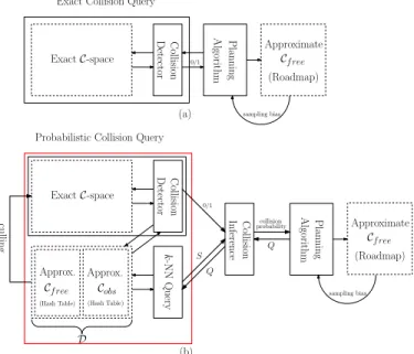
Exact collision checking is an important component of sampling-based motion planners. By providing binary collision statuses for configuration points or local paths in the config-uration space, collision checking helps the planners to learn about the connectivity ofC-space, and eventually to compute a collision-free continuous path connecting the initial and goal configurations in C-space (Figure 1(a)). The collision query results can also bias the planner’s sampling scheme through different heuristics (e.g., retraction rules).
Unlike the exact collision checking algorithm that computes many collision queries independently, our new probabilistic collision checking scheme exploits the prior collision infor-mation accumulated during the planning process, and lever-ages the spatial correlation between different collision queries (Figure 1(b)). In particular, after the collision checking routine finishes probing the C-space for a given query, we add the obtained information related to this query in a dataset D, which stores all the historical collision query results during the planning process. The stored information is a binary collision status, if the query is a point within C-space, or the collision statuses of several configuration points along the path, if the
ExactC-space
Collision
Detector Algorithm Planning
ExactC-space
Collision
Detector
Planning
Algorithm
k
-NN
Query
(b) (a)
Approximate
Cf ree
sampling bias
Approx.
Cf ree Approx.
Cobs
culling
0/1
(Roadmap)
(Hash Table) (Hash Table)
Approximate
Cf ree (Roadmap)
sampling bias
Exact Collision Query
Probabilistic Collision Query
Collision
Inference
Q
collision probability
Q S
D
0/1
Fig. 1:The collision detection module in sampling-based planners: exact collision checking only (a) and our approach with probabilistic collision checking (b). (a) The collision detection routine is an oracle
used by the planner to gather information about Cfree andCobs. The
planner performs binary collision queries, either on point
configura-tions or1-dimensional local paths, and estimates the connectivity of
Cfree(shown as ApproximateCfree). Moreover, some planners leverage in-collision results to bias sample generation according to different heuristics. (b) Our method also uses collision queries. However, we
store all in-collision results (as ApproximateCobs) and collision-free
results (as Approximate Cfree). Given a new query, our algorithm
first performs ak-NN query on the given configuration or local path
and then computes a collision probability for this query. The motion planner then uses the collision probability as a heuristic to guide the exploration process in the configuration space.
query is a local path. The resulting dataset D constitutes
the complete set of information we know about C-space, all learned from collision checking routines. Therefore, we use D as an approximate description of the underlying C-space: Cobs and Cfree are represented by in-collision samples and
collision-free samples, respectively. We then use these samples to estimate the collision status for a new query. The estimation result is in a form of a probability value, i.e., the collision
probability(refer to Section V for details).
Given a new queryQ, either a point or a local path, we first perform k-NN search on the dataset D to find its neighbor
set S. The set S provides a rough description about the
Q
(a)
Q
(b)
x2 x1
(c) l
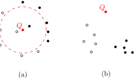
Fig. 2: Two types of k-NN queries used in our method: (a)
point-pointk-NN; (b) line-pointk-NN.Qis the query item, and the results
of different queries are shown as hollow circle points in each figure. We present novel LSH-based algorithms for fast computation of these
queries. (c) The line-point k-NN query is used to compute prior
collision instances that can influence the collision status of a local
path connecting x1 and x2 in C-space. The query line is the line
segment between x1 and x2. The white points are prior
collision-free samples in the dataset, and the black points are prior in-collision samples.
checking for a set of queries. For instance, many planners like RRT need to select a local path that can best improve the local exploration inCfree, i.e., a local path that is both long and
collision-free. The collision probability can be used to find an efficient sorting strategy, which thereby reduces the number of exact collision tests.
There are two types of k-NN queries involving in our
probabilistic collision checking algorithm. One retrieves points closest to a given point query: this is the well-known k-NN query, which we call thepoint-point k-NN query. The second query tries to find the points that are closest to a given line, which arises in the context of local path query. We call this second query the line-pointk-NN query. These two types of
k-NN queries are illustrated in Figure 2. For efficiency, both types of queries are implemented using the locality-sensitive hashing technique. For point-point k-NN queries, we directly build on prior LSH results in Section II-C. For line-point k -NN queries, we will present a new LSH-based algorithm in Section IV. When the collision result for a new configuration query is computed, we calculate the hash code for that query and add it to the hash tables. This operation is performed once for each item stored in the datasetD.
The notion of having sufficient information about S is
related to how confident we are about our inferences drawn from S. If the confidence is too small, the algorithm rejects the results of probabilistic collision queries and performs exact collision queries instead. We consider two types of rejection cases: ambiguity rejection and distance rejection (Dubuisson & Masson 1993). Ambiguity rejection happens when the collision probability of a given query is nearly 0.5. Distance rejection happens when the query configuration is far (in terms of geometric distance) from all prior instances stored in the database.
An overview of our probabilistic collision framework is given in Algorithm 1.
IV. LSH-BASEDLINE-POINTk-NN QUERY
One of the contributions of this paper is to extend the LSH formulation to the line-point k-NN query, for efficiently
Algorithm 1:probabilistic-collision-query(D, Q)
begin
ifQis point querythen
S←point-point-k-NN(Q)
ifSprovides sufficient information for inferencethen probabilistic-collision-query(S, Q)
else exact-collision-query(D, Q) ;
ifQis line querythen
S←line-point-k-NN(Q)
ifSprovides sufficient information for inferencethen probabilistic-continuous-collision-query(S, Q)
else exact-continuous-collision-query(D, Q) ;
estimating the collision status of a local path. In comparison with previous methods for such computations (Andoni et al. 2009, Basri et al. 2011), our line-point k-NN results in a more compact form. In addition, we also derive LSH bounds
similar to the point-point k-NN, as shown in Theorem 1.
Moreover, we address several issues that arise when using our algorithm for sampling-based motion planning, such as handling non-Euclidean metrics and reducing the dimension of the embedded space.
The simplest algorithm for line-pointk-NN query is based on sampling the line into a sequence of uniformly sampled points at a fixed resolution, and using point-pointk-NN algo-rithms on each of those sampled points. One major drawback of such an approach is its efficiency, as we land up performing a high number of point-point k-NN queries for a given line or local path. Furthermore, the samples in the database are typically not distributed in a uniform manner. As a result, it is hard to compute the appropriate sampling resolution for the line.
The main issue in terms of using LSH to perform line-point k-NN query is to embed the line query and the point dataset into a higher-dimensional space, and then to perform point-point k-NN queries in that embedded space. First, we present a technique to perform line-point embedding. Next, we design hash functions for the embedding and prove that these hash functions satisfy the locality-sensitive property for the original data (i.e., D). Finally, we derive the error bound
and time bound for the approximate line-point k-NN query,
which is similar to that given in Theorem 1.
A. Line-point Distance
A linelinRd is described asl=
{a+s·v}, whereais a point inRd onlandvis a unit vector inRd. The Euclidean
distance of a point x∈ Rd to the linel is:
dist2(x, l) = (x−a)·(x−a)−((x−a)·v)2. (2)
Given a database D ={x1, ...,xN} of N points in Rd, the
B. Line-point Embedding: Non-affine Case
We first assume the non-affine line query, i.e., l, passes through the origin (i.e., a = 0). In this case, dist(x, l) = x·x−(x·v)2, and it can be re-formalized as the inner product of two (d+ 1)2-dimensional vectors:
dist2(x, l) =x·x−(x·v)2 = Tr(xT(I
−vvT)x)
= Tr(
x
t
T
I 0T
(I−vvT) I 0
x
t
)
= Tr( I 0T
(I−vvT) I 0 x t x t T ) (3)
= vec( I 0T
(I−vvT) I 0 )·vec(
x t x t T )
=V(v)·V(x),
where I is d×d identity matrix, Tr(·) is the trace of a given square matrix andt can be any real value;vec(·)is the vectorization operation. VP(
·) is an embedding which yields a(d+1)2-dimensional vector fromd-dimensional point vector
x:VP(x) = vec(
x t x t T );VL(
·)is an embedding which yields a(d+ 1)2-dimensional vector from a linel={sv}in
d-dimensional space:VL(v) = vec(
I−vvT 0
0T 0
).
In addition, we notice that the Euclidean distance between
the embedding VP(x)and
−VL(v)is given by
kVP(x)
−(−VL(v))
k2 =d−1 +kVP(x)
k2+ 2(VP(x)
·VL(v))
=d−1 + (kxk2+t2)2+ 2 dist2 (x, l).
(4)
In Equation 4, if the term d−1 + (kxk2+t2)2 is constant, then the point-to-line distance dist(x, l) can be formalized
as the distance between two points VP(x) and
−VL(v)
in the higher-dimensional embedded space. This is possible because t is a free variable that can be chosen arbitrarily. In particular, we choosetas a function ofx:t(x) =p
c− kxk2, where c > maxx∈Dkxk2 is a constant real value related
to the entire database D but independent from each single
item in the database. In this way, Equation 4 reduces to kVP(x)
−(−VL(v))
k2= 2 dist2(x, l) +constant.
Until now, we have successfully separated the database item (i.e., x) from the query item (i.e., l). Next, we can pre-compute the locality-sensitive hash values for all the database items (see Section IV-D), which are used for efficient line-pointk-NN computation of any given line queries. Moreover, this reduction implies that we can reduce the line-point k
-NN query in a d-dimensional database D to a point k-NN
query in a(d+1)2-dimensional embedded databaseVP(
D) = {VP(x1), ..., VP(x
N)}, where the query item corresponds to
−VL(v).
C. Line-point Embedding: Affine Case
Now we consider the case of any arbitrary affine line, i.e., a6=0. Similarly to Equation 3, there is
dist2(x, l)
= (x−a)·(x−a)−((x−a)·v)2 = Tr((x−a)T(I
−vvT)(x
−a)) = Tr( x 1 t T
I −a 0T
(I−vvT) I
−a 0
| {z }
B x 1 t ) = vec( x 1 t x 1 t T
)·vec(B) (5)
= ˆV(x)·Vˆ(v,a),
whereVˆP(x)andVˆL(v,a)are(d+ 2)2-dimensional embed-dings for a point and line in Rd, respectively. Similarly to
Equation 4, if we choose t(x) = √c−x2−1, where c > maxx∈Dkxk2+ 1 is a constant related to the entire database D (i.e., set kVˆP(x)
k2 = c2), then dist2(x, l) also linearly depends on the squared Euclidean distance between the em-bedded database and the query item:kVˆP(x)
−VˆL(v,a)
k2=
c2 +d−2 + (dist2
(0, l) + 1)2+ 2 dist2
(x, l). As a result,
we can perform an affine line-point k-NN query based on
a point k-NN query in a (d + 2)2-dimensional database
ˆ
VP(
D) = {VˆP(x1), ...,VˆP(x
N)}, and the corresponding
query item is−VˆL(v,a).
The dimension of the embedded space (i.e.,(d+1)2or(d+ 2)2) is much higher than the original space (i.e., d), and will slow down the LSH computation. We present two techniques to reduce the dimension of the embedded space.
First, notice that the matrices used withinvec(·) are
sym-metric matrices. For a d ×d matrix A, we can define a
d(d+ 1)/2-dimensional embeddingvec(A)c as follows
c
vec(A) = [a√1,1
2, a1,2, ..., a1,d,
a2,2 √
2, a2,3, ...,
ad,d
√ 2]
T
. (6)
It is easy to see that kvec(A)−vec(B)k2 = 2k c vec(A)−
c
vec(B)k2 and hence this dimension-reduction will not influ-ence the accuracy of the line-pointk-NN algorithm introduced above.
Secondly, we can use the Johnson-Lindenstrauss lemma (Li et al. 2006) to reduce the dimension of the embedded data by randomly projecting the high-dimensional embedded data items onto a lower dimensional space. Compared to the first approach, this method can generate an embedding with lower dimensions, but according to our experimental results, it may reduce the accuracy of the line-pointk-NN algorithms.
D. Locality-Sensitive Hash Functions for Line-Point Query
We design the hash functionˆh for the line-point query as follows:
( ˆ
h(x) =h( ˆVP(x)), xis a database point
ˆ
h(l) =h(−VˆL(v,a)), l is a line
where h is a locality-sensitive hash function as defined in Section II-C. The new hash functions are locality-sensitive for line-point query, as shown by the following two theorems:
Theorem 2: The hash function family hˆ is (r, r(1 +
), p1, p2)-sensitive if his the hamming hash, (i.e., h=hu), where p1 = π1cos
−1(r2
C), p2 =
1
πcos
−1(r2(1+)2
C ) andC is
a value independent of database point, but is related to the query. Moreover, (1+1)2 ≤ρ=
logp1 logp2 ≤1.
Theorem 3: The hash function family hˆ is (r, r(1 +
), p1, p2)-sensitive if his the p-stable hash, (i.e., h=ha,b), where p1 = f(√2rW2+C) and p2 =f(
W
√
2r2(1+)2+C) and C is a value independent of database point, but is related to the query. The functionfis defined asf(x) = 1
2(1−2 cdf(−x))+ 1
√ 2πx(e
−1 2x
2
− 1), where cdf(x) = Rx −∞
1 √
2πe
−1 2t
2
dt is
a cumulative distribution function. Moreover, 1+1 ≤ ρ =
logp1 logp2 ≤1.
The proofs of Theorem 2 and Theorem 3 are provided in Appendix A and Appendix B.
Similarly to Theorem 1 for point-pointk-NN query, we can compute the error bound and time complexity for line-point
k-NN query as follows:
Theorem 4: (Line-pointk-NN query) LetHbe a family of
(r, r(1 +), p1, p2)-sensitive hash functions, with p1 > p2. Given a dataset of sizeN, we set the hash function dimension
M as M = log1/p2N and choose L = N
ρ hash tables,
where ρ = logp1
logp2. Using H along with L-hash tables over
M-dimensions, given a line queryl, with probability at least 1
2− 1
e, our LSH algorithm solves the(r, )-neighbor problem,
i.e., if there exists a point x that dist(x, l)≤r(1 +), then the algorithm will return the point with probability ≥ 12−1e. The retrieval time is bounded by O(Nρ).
The proof is given in Appendix C.
Theorem 4, along with Theorem 1, guarantees sub-linear time complexity when performingk-NN query on the histori-cal collision results, if hamming orp-stable hashing functions are applied.
V. PROBABILISTICCOLLISIONDETECTION BASED ON
k-NN QUERIES
In this section, we use the LSH-basedk-NN query presented in Section IV to estimate the collision probability for a given query. Our approach stores the outcome of prior instances of exact collision queries, including point queries and local path queries, within a database (shown as Approximate Cfree and
Approximate Cobs in Figure 1(b)). Those stored instances are
used to perform probabilistic collision queries.
A. Collision Status Classifier
Our goal is to estimate the collision probability for a query pointpor a query linelaccording to the database of previous collision query results. Based on the collision probability, we can design a classifier c(·) to predict the collision status of a given query. The expected prediction error for the classifier can be defined as
Eerror[c(p)| D]
=y(p)·P[c(p) = 0| D] + (1−y(p))·P[c(p) = 1| D]
and
Eerror[c(l)| D]
=y(l)·P[c(l) = 0| D] + (1−y(l))·P[c(l) = 1| D],
where D, as defined before, is a dataset of N points in Rd
andy(·)provides the exact collision status ofporl. A classifier is effectiveat predicting the collision status of point or line queries, if its prediction error will converge to zero when the size of databaseDincreases. In other words, an effective classifierc(·)should have the following properties:
lim
|D|→∞Eerror[c(p)| D] = 0or |D|→∞lim Eerror[c(l)| D] = 0. As we will show in Section V-E, if a collision status classi-fier is effective, our probabilistic collision detection algorithm can guarantee to converge to the exact collision results, as the size of the database increases.
B. Effective Classifier for Point Query
Here we give an example implementation of an effective collision status classifier. Following the previous work on locally-weighted regression (LWR) (Cohn et al. 1996, Burns & Brock 2005a), we fit a Gaussian distribution to the region surrounding a query point and then estimate the probability for collision, as well as the confidence of the estimation. The confidence is further used to determine whether there is sufficient information to infer the collision status of the query, as discussed in Section V-D.
The first case is the query point, i.e., the task is to compute
the collision status for a sample p in C-space. We first
perform point-pointk-NN query to compute the prior collision instances closest to p. Next, based on the collision status of the neighboring instances, the collision probability can be estimated as:
P[c(p) = 1| D] =E[c(p)| D] =µ2+ΣT12Σ −1
1 (p−µ1), (8)
and the variance of the estimation can be given as
Var[c(p)| D] (9)
= Σ2|1 (P
iwi)2
X
i
w2
i +F(p)
X
i
w2
iF(xi)
where µ1 =
P iwixi P
iwi , µ2 = P
iwiyi P
iwi = P
xi∈S\Cfreewi
P iwi ,
Σ1 = Piwi(xi−µ1)(xi−µ1)T
P
iwi , Σ2 = P
iwi(yi−µ2)2
P
iwi , Σ12 = P
iwi(xi−µ1)(yi−µ2)
P
iwi ,Σ2|1= Σ2−Σ
T
12Σ −1
1 Σ12, andF(x) =
(x−µ1)TΣ−1
1 (x−µ1).S is the neighborhood set computed using point-pointk-NN query andyi=y(xi)is the exact
col-lision status of instancexi.wi=e−γdist(xi,p)is the
distance-tuned weight for each k-NN neighbor xi. The parameter γ
controls the magnitude of the weightwi, which measures the
correlation between the labels of xi and query point p. In
all our experiments, γ is set according to the scale of the environment (e.g., the diameter of the bounding sphere for the environment):
Once the collision probabilityP[c(p) = 1| D]is computed,
we can predictp’s collision status using an appropriate thresh-old t∈ (0,1): when P[c(p) = 1| D] > t, we classify p as
in-collision; otherwise, we classify it as collision-free. This classifier is effective for anyt∈(0,1), because when the size of D increases, if pis actually in-collision (i.e., y(p) = 1),
more and more points in its neighborhood S will be inside
Cobs, and thereforeP[c(p) = 1| D] converges to1. Similarly, P[c(p) = 1| D] will converge to0 ifpis actually
collision-free. As a result, given a large enough database, the classifier can always correctly predict the query point’s collision status and is thus effective.
C. Effective Classifier for Local Path Query
The second case is the line query. The goal of the line query is to estimate the collision status of a local path in C-space. We require the local path to lie within the neighborhood of the line segmentl connecting its two endpoints, i.e., the local path should not deviate too much from l. The first step is to perform a line-point k-NN query to find the prior point collision query configurations closest to the infinite line thatl
lies on. Next, we need to filter out the points whose projections are outside the truncated segment ofl, as shown in Figure 2(c). This process might trim down some samples that are very close to the line, but lie just beyond the segment l along the axis of the line. Since these samples are isolated from the line segment by the segment’s two end-points, the collision status of the segment is independent with the collision status of these samples, given that the segment’s two end-points are collision-free. As a result, not considering these samples does not change the outcome of the line query. Finally, we apply our inference method (as shown below) on the filtered results, denoted as S, to estimate the collision probability of the local path.
One way to compute the collision probability for a line is to use LWR (Burns & Brock 2005a). The collision probability can be estimated as:
P[c(l) = 1| D] =E(c(l)| D] (11)
=µ2+ΣT12Σ −1
1 (NearestPnt(l,µ1)−µ1),
and
Var[c(l)| D] (12)
= Σ2|1 (P
iwi)2
X
i
w2
i +F(NearestPnt(l,µ1))
X
i
w2
iF(xi).
where the symbols are as defined in Equation 8 and Equa-tion 12, except the terms related withwi, which is now defined
as wi = e−γdist(xi,l). Function NearestPnt(l,x) returns a
point on line segment l that is closest to a pointx.
However, the above LWR-based method has some limita-tions. The main issue is that it can only compute a collision probability for the entire line. In many cases, we need to know where the collision is likely to happen on the line (i.e., the first time of contact (TOC)). We provide an optimization method for estimating the approximate TOC. In particular, we divide the line l into I segments and assign each segment, say li,
a label ci to indicate its collision status. We aim to find a
suitable label assignment{c∗
i}Ii=1 so that:
{c∗
i}= argmin{ci}∈{0,1}I
I
X
i=1
(ci−c0i)2+κ I−1 X
i=1
(ci−ci+1)2,
wherec0iis the collision status for the midpoint ofliestimated
using Equation 8. The term (ci−c0i)2 constrains the label
assignment to be consistent with point query results, and PI−1
i=1(ci −ci+1)2 is a smoothness term, which models the
fact that collision labels for adjacent points are likely to be the same. Parameterκadjusts the relative weight between the consistency term and the smoothness term. The optimization can be computed efficiently using dynamic programming. After that, we can estimate the collision probability for the line as
P[c(l) = 1| D] =E[c(l)| D] = max
i: c∗ i=1
c0i, (13)
and the approximate first time of contact can be given as mini: c∗
i=1i/I.
Based on the collision probability formulated as above, we can design a classifier to predict the collision status for a given line query by using a specific threshold t ∈(0,1) to justify whether the query is in-collision or not. If the query’s collision probability is larger thant, we return in-collision; otherwise, we return collision-free. This classifier is also effective for any t ∈(0,1), because when the size of D increases, if l is in-collision, there always exists one segment li on l whose
collision probability c0
i converges to 1 and thereforeP[c(l) =
1| D] will converge to1. Similarly, if l is collision-free, the probability will converge to0.
Remark The collision status classifiers described above are generative classifiers, i.e., they are constructed after the con-ditional collision probability is computed. One advantage of the generative classifier is that it can be used even in a dynamic environment where the obstacles may change their positions. However, in our approach, we only need to know the binary collision status of the query instead of its collision probability. As a result, we can use effectivediscriminativeclassifiers, i.e., design a classifier directly from the data. For example, we can use the weighted average of the query’s neighbors’ collision status to predict the query’s collision status; then all we need to learn are those weight factors. Given a large database of historical data, a discriminative classifier is usually more robust than a generative classifier. However, the discriminative classifier is specific to the current database, and the need to learn a new classifier when the environment changes can be expensive. The discriminative classifier is thus limited to static environments.
D. Rejection Rules
Q
(a)
Q
(b)
Fig. 3: Two rejection rules: (a) ambiguity rejection:Q’s estimated
collision probability is near 0.5 or the variance for the estimate is
large; (b) distance rejection: whenQis far from all in-collision and
collision-free database items.
We consider two types of rejection rules (Dubuisson & Masson 1993):ambiguity rejectionanddistance rejection.
• Ambiguity rejection happens when the estimated collision status is ambiguous. For instance, suppose there are the same number of in-collision points and collision-free points in the neighborhood of a point queryp, and these points all lie same distance from the query. The collision probability computed by Equation 8 is 0.5 in this case; therefore any estimate of the collision status is equivalent to a random guess. Ambiguity also occurs when the variance of the estimated collision status (computed by Equation 9) is large. To determine whether ambiguity rejection is necessary for a point query p, we measure the ambiguity as
Amb= min(E[c(p)],1−E[c(p)])2+Var[c(p)],
whereE[c(p)] and Var[c(p)]are computed according to Equation 8 and Equation 9. If Ambis larger than a given thresholdAd, we reject the estimate and perform the exact
collision test.
• Distance rejection happens when the k-NN points for a given query lie too far away from the query configuration (in terms of the distance). This is a problem because our collision status estimator is based on coherency of nearby points’ or lines’ collision statuses. This distance rejection happens when the database is nearly empty, or when the query is in a region not well sampled by current configuration database. In order to determine whether we need to perform distance rejection, we compute Dis, the distance frompto its nearest point. IfDisis larger than a given threshold Dd (for instance, Disis ∞ when the
database is empty), we perform the exact collision query.
The two rejection rules are shown in Figure 3. The rejection rules for a line query are similar.
E. Asymptotic Property of Probabilistic Collision Query
If the classifier used in the probabilistic collision query is effective, we can prove that the collision status returned by the probabilistic collision checking module will converge to the exact collision detection results when the size of the dataset increases (asymptotically):
Theorem 5: The collision query performed using
LSH-based k-NN will converge to the exact collision detection as the size of the dataset increases.
Proof:We only need to prove that both the probability of
a false positive (i.e., returns in-collision status when there is in fact no collision) and a false negative (i.e., returns collision-free when there is in fact a collision) converges to zero, as the size of the database increases.
Given a query, we denote itsr-neighbor asBr, wherer is
the distance between the query and its k-th nearest neighbor. For a point query, Br is an r-ball around it. For a line
query, Br is the set of all points with distance r to the line
(i.e., a line swept-sphere volume). Let P1 =
µ(Br(1+)∩Cobs) µ(C-space)
and P2 =
µ(Br(1+)∩Cfree)
µ(C-space) , which are the probabilities that a uniform sample inC-space is in-collision or collision-free and within query’sr(1+)-neighborhood. Hereµ(·)is the volume measure. LetN be the size of the database corresponding to the prior instances.
A false negative occurs if and only if the following two cases are true: 1) there are no in-collision points within Br(1+), and therefore the probabilistic method always returns collision-free; 2) there are in-collision points within Br(1+), but the classifier predicts wrong label.
First, we compute the probability for case 1. The event that there are no in-collision points within Br(1+) happens either when no dataset point lies withinBr(1+)or when there exist some points within that ball which are missed due to the
approximate nature of LSH-based k-NN query. According to
Theorem 1, we have
P[case 1]
=
N
X
i=0
N i
(1−P1)N−iPi
1(1−(1/2−1/e))i
= (1−P1(1/2−1/e))N
→0 (asN → ∞).
Case 2 can occur when case 1 does not happen and the classifier gives the wrong results. However, as the classifier is effective, we have
P[case 2]
= (1−P[case 1])·Perror[xor l in-collision;D]
= (1−P[case 1])·Eerror[c(x)or c(l)| D]
→0 (as N → ∞).
As a result, we have
P[false negative] =P[case 1] +P[case 2]→0 (asN → ∞).
Similarly, a false positive occurs if there are no collision-free points withinBr(1+)or if there are collision-free points within Br(1+) but the classifier still predicts a wrong label. The probability of case 1 can be given as
P[case 1] = (1−P2(1/2−1/e))N
and the probability of case 2 is
P[case 2] = (1−P[case 1])·Perror[xor l collision free;D]
Both terms converge to zero when the size of the database increases. As a result, we can conclude that the false positive also converges to0:
P[false positive] =P[case 1] +P[case 2]→0 (asN → ∞).
Remark Note that the convergence of the collision query
using LSH-based k-NN query is slower than that using the
exact k-NN based method, whose prediction errors can be
given as:P[false negative] = (1−P1)N andP[false positive]≤
(1−P2)N.
Remark The fact that the probability of getting false negative (or false positive) converges to 0is true if and only ifP1 (or
P2) is not0. Usually we assume that real world obstacles are compact and therefore obstacles inC-space are also compact. Thus, if a configuration is collision-free, there is an open set surrounding it that is collision-free as well and therefore
P2 > 0. However, a configuration in-collision (i.e., inside a contact set) does not necessarily have a positive P1 (i.e., P1 may be zero). As these kinds of ‘bad’ configurations are of zero measure, our proof of Theorem 5 still holds.
VI. ACCELERATINGSAMPLING-BASEDPLANNERS
In this section, we first discuss techniques to accelerate various sampling-based planners using our probabilistic col-lision query, including 1) how the database is constructed and maintained; 2) how to accelerate various planners; 3) how to handle dynamic environments; 4) how to combine these techniques with non-uniform sampling techniques. Next, we analyze the factors that can influence the performance of resulting planners using our probabilistic collision queries. Finally, we prove the completeness and optimality of modified sampling-based planners.
A. Database Construction
When the planner thread starts, the database of prior colli-sion query results is empty. Given a point query, we first com-pute itsk-nearest neighboring pointsS. Based onS, we check whether distance rejection is necessary. If so, we perform exact collision test and add the query result into the database. Otherwise, we estimate the query’s collision probability and the confidence of our estimate, using approaches discussed in Section V. Next, we check for ambiguity rejection. Based on the outcome of ambiguity rejection, we may again perform exact collision query and add the result to the database; or the estimated collision result can be directly used by a sampling-based planner. When a local path query is given, the processing pipeline is similar, except that when performing exact collision checking of the local path, a series of point configurations on the local path are added to the database. In summary, we perform exact collision tests only for queries that are located within regions that are not well covered by the current database D; the resulting query results are added into D. Later, in Section VI-B, we verify the collision status of a query using exact collision test when it is estimated as collision-free. This test is performed to guarantee the overall motion planning
algorithm to be conservative. However, such queries are not added to the database.
Next, we discuss the efficiency of operations on the LSH-based database, which is implemented as a hash table. The hash table starts out empty, so there is no pre-processing overhead. When we decide to add the result for a collision query xinto the database, we first compute its hashing code ˆ
h(x)and then add it into the hash table. This step’s complexity
remains constant. After warm-up, we begin performingk-NN
query on the hash table, which has the complexityO(Nρ)(all
symbols are as defined in Theorem 4). After addingN items
into the hash table and performing ∼
N probabilistic collision queries, the overall complexity of the database operations
becomesO(N+N∼·Nρ). Note that the number of all collision
queries is larger than max(N,N∼); therefore the amortized computational overhead on each collision query isO(1).
B. Accelerating Various Planners
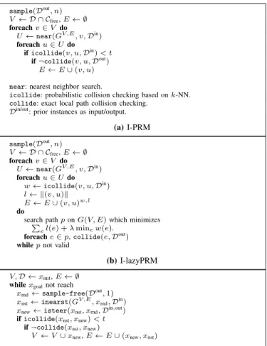
Algorithm 1 highlights our basic approach to apply the probabilistic collision query: we use the computed collision probability as a filter to reduce the number of exact collision queries. If a given configuration or local path query is close to in-collision instances, then it has a high probability of being in-collision. Similarly, if a query has many collision-free instances around it, it is likely to be collision-collision-free. In our implementation, we cull away only those queries with high collision probabilities. For queries with high collision-free probability, we still perform exact collision tests on them in order to guarantee that the overall collision detection algorithm is conservative. In Figure 4(a), we show how our probabilistic culling strategy can be integrated with the PRM algorithm by only performing exact collision checking (collide) for queries with collision probability (icollide) larger than a given threshold t. Note that the neighborhood search routine (near) can use LSH-based point-pointk-NN query.icollide is computed according to Equation 8 or Equation 11.
In Figure 4(b), we show how to use the collision probability as a cost function with the lazyPRM algorithm (Kavraki et al. 1996). In the basic version of lazyPRM algorithm, the expensive local path collision checking is delayed till the search phase. The basic idea is that the algorithm repeatedly searches the roadmap to compute the shortest path between the initial and goal nodes, performs collision checking along the edges, and removes the in-collision edges from the roadmap. However, the shortest path usually does not correspond to a collision-free path, especially in complex environments. We improve the lazyPRM planner using probabilistic colli-sion queries. We compute the collicolli-sion probability for each roadmap edge during roadmap construction, based on Equa-tion 13. The probability (w) as well as the length of the edge (l) are stored as costs of the edge. During the search step, we try to compute the shortest path with a minimum collision probability, i.e., a path that minimizes the cost P
el(e) +λminew(e), where λis a parameter that controls
A. Database Construction
When the planner thread starts, the database of prior colli-sion query results is empty. Given a point query, wefirst com-pute itsk-nearest neighboring pointsS. Based onS, we check
whether distance rejection is necessary. If so, we perform exact collision test and add the query result into the database. Otherwise, we estimate the query’s collision probability and the confidence of our estimate, using approaches discussed in Section V. Next, we check for ambiguity rejection. Based on the outcome of ambiguity rejection, we may again perform exact collision query and add the result to the database; or the estimated collision result can be directly used by a sample-based planner. When a local path query is given, the processing pipeline is similar, except that when performing exact collision checking of the local path, a series of point configurations on the local path are added to the database. In summary, we perform exact collision tests only for queries that are located within regions that are not well covered by the current database D; the resulting query results are added into D. Later, in Section VI-B, we verify the collision status of a query using exact collision test when it is estimated as collision-free. This test is performed to guarantee the overall motion planning algorithm to be conservative. However, such queries are not added to the database.
Next, we discuss the efficiency of operations on the LSH-based database, which is implemented as a hash table. The hash table starts out empty, so there is no pre-processing overhead. When we decide to add the result for a collision queryx into the database, we first compute its hashing code
ˆ
h(x)and then add it into the hash table. This step’s complexity
remains constant. After warm-up, we begin performingk-NN
query on the hash table, which has the complexityO(Nρ)(all symbols are as defined in Theorem 4). After addingN items into the hash table and performing M probabilistic collision
queries, the overall complexity of the database operations becomesO(N+M·Nρ). Note that the number of all collision queries is larger than max(N, M); therefore the amortized
computational overhead on each collision query isO(1).
B. Accelerating Various Planners
Algorithm 1 highlights our basic approach to apply the probabilistic collision query: we use the computed collision probability as a filter to reduce the number of exact collision queries. If a given configuration or local path query is close to in-collision instances, then it has a high probability of being in-collision. Similarly, if a query has many collision-free instances around it, it is likely to be collision-collision-free. In our implementation, we cull away only those queries with high collision probabilities. For queries with high collision-free probability, we still perform exact collision tests on them in order to guarantee that the overall collision detection algorithm is conservative. In Figure 4(a), we show how our probabilistic culling strategy can be integrated with the PRM algorithm by only performing exact collision checking (collide) for queries with collision probability (icollide) larger than a given threshold t. Note that the neighborhood search routine
sample(Dout, n)
V ←D∩Cfree,E← ∅
foreachv∈V do U←near(GV,E, v,
Din)
foreachu∈Udo
ificollide(v, u,Din)< t if¬collide(v, u,Dout)
E←E∪(v, u)
near: nearest neighbor search.
icollide: probabilistic collision checking based onk-NN. collide: exact local path collision checking.
Din/out: prior instances as input/output. (a)I-PRM
sample(Dout, n)
V ←D∩Cfree,E← ∅
foreachv∈V do U←near(GV,E, v,
Din)
foreachu∈Udo w←icollide(v, u,Din)
l← �(v, u)� E←E∪(v, u)w,l
do
search path� ponG(V, E)which minimizes el(e) +λminew(e).
foreache∈p,collide(e,Dout)
whilepnot valid
(b)I-lazyPRM
V,D←xinit,E← ∅
whilexgoalnot reach
xrnd←sample-free(Dout,1)
xnst←inearst(GV,E, x
rnd,Din)
xnew←isteer(xnst, xrnd,Din,out)
ificollide(xnst, xnew)< t if¬collide(xnst, xnew)
V←V∪xnew,E←E∪(xnew, xnst)
inearest:find the nearest tree node that has high collision-free probability. isteer: steer from a tree node to a new node, usingicollidefor validity checking.
(c)I-RRT
V,D←xinit,E← ∅
whilexgoalnot reach
xrnd←sample-free(Dout,1)
xnst←inearst(GV,E, x
rnd,Din)
xnew←isteer(xnst, xrnd,Din,out)
ificollide(xnst, xnew)< t if¬collide(xnst, xnew)
V←V∪xnew
U←near(GV,E, x new)
foreachx∈U, compute weightc(x) =
λ�(x, xnew)�+icollide(x, xnew,Din) sortUaccording to weightc.
Letxminbe thefirstx∈Uwith¬collide(x, xnew)
E←E∪(xmin, xnew)
foreachx∈U,rewire(x)
inearest:find the nearest tree node that has high collision-free probability. isteer: steer from a tree node to a new node, usingicollidefor validity checking. rewire: RRT∗routine used to update the tree topology for optimality guarantee.
(d)I-RRT∗
Fig. 4: Our probabilistic collision checking module can improve
a wide variety of motion planners. Here we present four modified
planners as example.
Fig. 4: Our probabilistic collision checking module can improve a wide variety of motion planners. Here we present four modified planners as example.
account based on collision probability, the resulting path is more likely to be collision-free.
Finally, the collision probability can be used by the motion planner to explore Cfree in an efficient manner. We use RRT
to illustrate this benefit (Figure 4(c)). Given a random sample
xrnd, RRT computes a node xnst among the prior collision-free configurations that are closest to xrnd and expands from
xnst towards xrnd. If there is no obstacle in C-space, this exploration technique is based on the Voronoi heuristic that biases the planner towards the unexplored regions. However, the existence of obstacles affects its performance: the planner may run into Cobs shortly after expansion, and the resulting
exploration is limited. Using thek-NN based inference, we can estimate the collision probability for local paths connecting
xrndwith each of its neighbors and choosexnstas the one with both a long edge length and a small collision probability (i.e.,
xnst= argmax(l(e)−λ·w(e)), where λis a parameter used to control the relative weight of these two terms). A similar strategy can also be used for RRT∗, as shown in Figure 4(d).
C. Narrow Passages and Non-uniform Samples
Narrow passages are a key issue for sampling-based motion planners. In general, it is difficult to generate enough number of samples in the narrow passages and capture the connectivity of the free space. Narrow passages can lead to some additional issues in terms of the collision status classifier presented in SectionV-B. In narrow passages, a collision-free query point configuration can be wrongly classified as in-collision, as shown in Figure 5. This is because the collision status inference algorithm assumes the spatial coherency about the collision status, i.e., nearby samples in theC-space tend to have the same collision status. However, such spatial coherency may not work in the regions around narrow passages and this may reduce the accuracy of collision status estimated via the inference algorithm. This reduced accuracy can also decrease the performance of the sampling-based planner in narrow passages. If a random planner can indeed generate a free-space sample in the narrow passage, the inference algorithm may incorrectly classify it as in-collision and may not add it to the
database D and the roadmap/tree-structure computed by the
planner. As a result, the planner may not be able to capture the connectivity of the space correctly around that narrow passage.
Q
Fig. 5: Q is a collision-free query point configuration inside the narrow passage, but the collision status classifier may estimate it as in-collision, because all its nearby samples in the database (shown as black dots) are all in-collision.
collision test, even when the inference algorithm estimates the query to have a large collision probability. In particular, suppose the estimated collision probability of a query is p, wherep∈(0.5,1], then with a probability ofmax(1−p, ps),
we check the exact collision status of the query, wherepsis a
small value (e.g.,0.01). In practice, this occasional verification strategy works well on narrow passage benchmarks and pro-vides a good trade-off between efficiency and completeness.
However, for some narrow passages with small expan-siveness, defined based on the criteria in (Hsu et al. 1997), this occasional verification with an exact collision test can slowdown the process of generating sufficient number of samples in the narrow passages, which affects the perfor-mance of probabilistic collision checking. In order to handle challenging narrow passage scenarios, we combine the non-uniform sampling strategies used in different sampling-based planners (Boor et al. 1999, Rodriguez et al. 2006, Sun et al. 2005) with our probabilistic collision query to quickly generate
more narrow passage samples in the database D and the
planner’s roadmap. In particular, with a probability of 1−ps,
we perform uniform sampling using probabilistic collision checking; with a probability of ps, we perform non-uniform
sampling with exact collision checking to increase the number of samples in the narrow passages. The samples generated by non-uniform sampling are directly added into the database and are used later by the inferencing algorithm.
D. Performance Analysis
The modified planners are faster, mainly because we replace some of the expensive, exact collision queries with relatively cheap k-NN queries. Let the timing cost for a single exact collision query be TC and for a single k-NN query be TK,
where TK < TC. Suppose the original planner performs C1 collision queries and modified planners performsC2 collision queries andC1−C2 k-NN queries, whereC2< C1. We also assume that the two planners spend the same timeAon other computations within a planner, such as sample generation, maintaining the roadmap or the tree structure, etc. Then the speedup ratio obtained by the modified planner is:
R= TC·C1+A
TC·C2+TK·(C2−C1) +A
. (14)
Therefore, if TC TK and TC ·C1 A, we have R ≈
C1/C2, i.e., if the higher number of exact collision queries are culled, we can obtain a higher speedup. The extreme speedup ratio C1/C2 may not be reached, however, for two reasons.
1) TC·C1 Amay not hold, such as when the underlying
collision-free path solution lies in some narrow passages (A
is large) or in open spaces (TC·C1 is small); or 2)TC TK
may not hold, such as when the environment and robot have low geometric complexity (i.e., TC is small) or the instance
dataset is large and the cost of the resulting k-NN query is high (i.e.,TK is large).
Note that R is only an approximation of the actual
ac-celeration ratio. It may overestimate the speedup, because a collision-free local path may have a collision probability
higher than a given threshold; our probabilistic collision ap-proach filters such high probabilities out. If such a collision-free local path is critical for the connectivity of the roadmap, such false positives due to the probabilistic collision checking module will cause the resulting planner to perform more exploration, and thereby increases the overall planning time. As a result, we need to choose an appropriate threshold that can provide a balance: we need a large threshold to filter out more collision queries and increase R; at the same time, we need to use a small threshold to reduce the number of false positives. However, the threshold choice is not important in the asymptotic sense. According to Theorem 5, the false positive error converges to0 when the database size increases.
R may also underestimate the actual speedup, because the timing cost for different collision queries can be different. For configurations near the boundary ofCobs, the collision queries
are more expensive. Therefore, the timing cost of checking the collision status for an in-collision local path is usually larger than that of checking a collision-free local path, because the former always has one configuration on the boundary of Cobs. As a result, it is possible to obtain a speedup larger than C1/C2.
E. Completeness and Optimality
As a natural consequence of Theorem 5, we can prove the probabilistic completeness and optimality of the new planners. To avoid the narrow passage problems, while discussing the new planners’ completeness, we assume that they apply the heuristics mentioned in Section VI-C. In other words, we assumeps>0 in order to guarantee that the critical samples
in the narrow passage will not be filtered out by mistake.
Theorem 6: I-PRM and I-lazyPRM are probabilistically
complete. I-RRT∗is probabilistically complete and asymptot-ically optimal.
Proof:A motion planner MP is probabilistically complete
if its failure probability, i.e., when a collision-free path exists, the probability that it cannot find a solution afterN samples
converges to 0 when the number of samples N increases:
limN→∞P[MP fails] = 0, where[MP fails]denotes the event
that the motion planner fails to find a solution afterN samples, when the solution exists.
Suppose we replace MP’s exact collision detection query by the probabilistic collision query and denote the new planner as I-MP. I-MP can fail in two cases: 1) MP fails; 2) MP computes a solution but some edges on the collision-free path are classified as in-collision by our collision status inference algorithm (i.e., false positives). LetLbe the number of edges in the solution path and letEi denote the event that the i-th
edge is incorrectly classified as in-collision. As a result, we have
P[I-MP fails]
=P[MP fails] + (1−P[MP fails])·P[
L
[
i=1
Ei]
≤P[MP fails] +
L
X
i=1