78:7–4 (2016) 7–14 | www.jurnalteknologi.utm.my | eISSN 2180–3722 |
Jurnal
Teknologi
Full Paper
VELOCITY CONTROL OF A UNICYCLE TYPE OF
MOBILE
ROBOT
USING
OPTIMAL
PID
CONTROLLER
Norhayati A. Majid, Z. Mohamed
*, Mohd Ariffanan Mohd Basri
Faculty of Electrical Engineering, Universiti Teknologi Malaysia, 81310
UTM Johor Bahru, Johor, Malaysia
Received
15 December 2015
Received in revised form
30 March 2016
Accepted
30 May 2016
*Corresponding author
[email protected]
Graphical abstract
Abstract
A unicycle model of control a mobile robot is a simplified modeling approach modified from the differential drive mobile robots. Instead of controlling the right speed, 𝑉𝑅 and the left speed, 𝑉𝐿 of the drive systems, the unicycle model is using 𝑢 and 𝜔 as the controller parameters. Tracking is much easier in this model. In this paper, the dynamic of the robot parameter is controlled using two blocks of Proportional-Integral-Derivative (PID) controllers. The gains of the PID are firstly determined using particle swarm optimization (PSO) in offline mode. After the optimal gain is determined, the tracking of the robot’s trajectory is performed online with optimal PID controller. The achieved results of the proposed scheme are compared with those of dynamic model optimized with genetic algorithm (GA) and manually tuned PID controller gains. In the algorithm, the control parameters are computed by minimizing the fitness function defined by using the integral absolute error (IAE) performance index. The simulation results obtained reveal advantages of the proposed PSO-PID dynamic controller for trajectory tracking of a unicycle type of mobile robot. A MATLAB-Simulink program is used to simulate the designed system and the results are graphically plotted. In addition, numerical simulations using 8-shape as a reference trajectory with several numbers of iterations are reported to show the validity of the proposed scheme.
Keywords: Unicycle type of mobile robot, tuning dynamic gains, PSO-PID controller
© 2016 Penerbit UTM Press. All rights reserved
1.0 INTRODUCTION
A simplified control model called unicycle type of mobile robots has been used in many robotics applications. There are many proposed control laws in the mobile robot literature that can be used to control a unicycle type of mobile robots. One of the approaches used to design the basic control laws is based on kinematic and dynamic [1]. Most of the latest design has considered the dynamic part to improve the robot performance in the real condition. For example, Martin et al. [2] has considered using
adaptive dynamic controller with feedback
linearization. This control approach has good performance, however, it is dependent on accurate
model parameters, i.e. when model parameters are unknown, adaptive control for adjusting these parameters is required. Some authors used backstepping techniques to design the adaptive control law [3]. Although the backstepping method can provide a systematic process, the controller parameters are obtained arbitrarily. On the other hand, other authors have used a feedback linearization approach and Lyapunov theories [4]. The saturation feedback controller for unicycle mobile robot proposed by Lee et al. [5], however, it is only applicable for a single controller. Thus, a kinematic controller, which controls the trajectory of the robot at an upper level, and an adaptive dynamic controller, which controls the velocities of the robot at a lower
level is necessary. The previous work done by Martin et al. [6] described the controller gains of the unicycle dynamic model adjusted using genetic algorithms.
However, GA performance indicates slow
convergence.
In this paper, an extension of the above work on velocity controller by using PID is developed. PID gains such as 𝐾𝑝 𝐾𝑖 and 𝐾𝑑 are determined by the
controllers, however, the three adjustable controller parameters should be tuned appropriately. The existence of conventional parameter tuning techniques such as Ziegler-Nichols (ZN) and various artificial intelligence approaches such as Genetic Algorithm (GA), Artificial Neural Network (ANN), Ant Colony Optimization (ACO) and Differential Evolutions (DE) could help to tune the PID for optimal gain combinations for a better response of the system.
More recently, an optimization technique, Particle Swarm Optimization (PSO) has been introduced. A comparative study between PSO and GA has been carried out by Hassan et al. [7] and it was found that PSO gives better performance as it has good global searching ability and easier to be implemented than GA. However, as PSO is a new evolutionary computation technique, there are not many research have been done yet in implementing PSO technique in dynamic model of unicycle mobile robot. A good example of using PSO-PID is reported by Hashim et al. [8] utilized on precise positioning system in micro-EDM specific for biomedical application where the PI and PID controllers are used to control the DC motor precisely.
This paper will be focused on employing optimal PID controller into the dynamic model of the unicycle-like mobile robot that will be explained in Section 2. The method of tuning PID controller is discussed in Section 3. Next, Section 4 presents the simulation setup via MATLAB-SIMULINK. Section 5 highlights the results, of comparative studies between the proposed controller and the controller designed by the Martin et al. [6]. Lastly, the Section 6 concludes the results and the findings.
2.0 ROBOT MODEL
A unicycle mobile robot considered in this paper is a class of nonholonomic mobile robots. Therefore it also has nonholonomic constrains due to the wheel limitations. In this section, the dynamic model of the unicycle-like mobile robot proposed by Martin et al. [1] is reviewed. Figure 1 depicts the mobile robot, its parameters and variables of interest. 𝒖 and 𝝎 are the linear and angular velocities of the robot, respectively, 𝑮 is the center of mass of the robot, 𝑪 is the position of the castor wheel, 𝑬 is the location of a tool onboard the robot, 𝒉 is the point of interest with coordinates 𝑥 and 𝑦 in the XY plane, ψ is the robot orientation, and a is the distance between the point of interest and the central point of the virtual axis linking the traction wheels (point B).
Figure 1 The differential drive (unicycle-like) mobile robot [2] 2.1 Kinematic Modeling
The design of the kinematic controller is based on the kinematic model of the robot, assuming that the disturbance term in Eq. (1) is a zero vector. From Martin et al. [2], the robot’s kinematic model is given by
[ 𝑥̇ 𝑦̇ 𝜓̇ ] = [ 𝑐𝑜𝑠 𝜓 − a sin 𝜓 sin 𝜓 a cos 𝜓 0 1 ] [𝜔𝑢], (1)
whose output are the coordinates of the point of interest, thus meaning 𝐡 = [𝑥 𝑦]𝑇. Hence
𝐡̇ = [𝑥̇𝑦̇] = [cos 𝜓 −𝑎 sin 𝜓 sin 𝜓 𝑎 cos 𝜓] [ 𝑢 𝜔] = 𝐴 [ 𝑢 𝜔] (2) with 𝐴 = [cos 𝜓 −𝑎 sin 𝜓
sin 𝜓 𝑎 cos 𝜓] whose inverse is 𝐴−1= [ cos 𝜓 sin 𝜓 −1 𝑎sin 𝜓 1 𝑎cos 𝜓 ]
Therefore, the inverse kinematics is given by [𝜔𝑢] = [ cos 𝜓 sin 𝜓 −1 𝑎sin 𝜓 1 𝑎cos 𝜓 ] [𝑥̇𝑦̇] (3) and the kinematic control law proposed to be applied to the robot is given by
[𝑢𝑟𝑒𝑓 𝑐 𝜔𝑟𝑒𝑓𝑐 ] = [ cos 𝜓 sin 𝜓 −1 𝑎sin 𝜓 1 𝑎cos 𝜓 ] [ 𝑥𝑑̇ + 𝐼𝑥 𝑡𝑎𝑛ℎ ( 𝑘𝑥 𝐼𝑥𝑥̃) 𝑦𝑑̇ + 𝐼𝑦 𝑡𝑎𝑛ℎ ( 𝑘𝑦 𝐼𝑦𝑦̃) ] (4)
Instantaneous distance error can be calculated as 𝑒(𝑡) = √𝑥̃2+ 𝑦̃2 (5)
where, 𝑥̃ = 𝑥𝑑− 𝑥, and 𝑦̃ = 𝑦𝑑− 𝑦 are the current
position errors in the axes X and Y, respectively, 𝑘𝑥> 0
𝐼𝑦∈ ℜ are saturation constants, and (𝑥, 𝑦) and (𝑥𝑑, 𝑦𝑑)
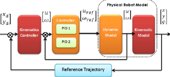
are the current and the desired coordinates of the point of interest, respectively. The objective of such a controller is to generate the references of linear and angular velocities for the dynamic controller, as shown in Figure 2.
Figure 2 Overall PID control system 2.2 Dynamic Modeling
The complete mathematical model adopted from De
La Cruz and Carelli [9), is written as
[ 𝑥̇ 𝑦̇ 𝜓̇ 𝑢̇ 𝜔̇] = [ 𝑢𝑐𝑜𝑠𝜓 − 𝑎𝜔𝑠𝑖𝑛𝜓 𝑢𝑠𝑖𝑛𝜓 + 𝑎𝜔𝑐𝑜𝑠𝜓 𝜔 𝜃3 𝜃1𝜔 2−𝜃4 𝜃1 −𝜃5 𝜃2𝑢𝜔 − 𝜃6 𝜃2𝜔 ] + [ 0 0 0 0 0 0 1 𝜃1 0 0 1 𝜃2] [𝜔𝑢𝑟𝑒𝑓 𝑟𝑒𝑓] + [ 𝛿𝑥 𝛿𝑦 0 𝛿𝑢 𝛿𝜔] , (6)
where 𝑢𝑟𝑒𝑓 and 𝜔𝑟𝑒𝑓 are the desired values of the
linear and angular velocities, respectively, representing the input signals for the system. A vector of identified parameters and a vector of parametric uncertainties are associated with the above model of the mobile robot, which are,
𝛉 = [𝜃1 𝜃2 𝜃3 𝜃4 𝜃5 𝜃6]𝑇 (7)
and
𝛅 = [𝛿𝑥 𝛿𝑦 0 𝛿𝑢 𝛿𝜔]𝑇 (8)
where 𝛿𝑥 and 𝛿𝑦 are functions of the slip velocities and
the robot orientation, 𝛿𝑢 and 𝛿𝜔 are functions of
physical parameters as mass, inertia, diameters of the wheel and tyre, parameters of the motors, forces on the wheels, etc., are considered as disturbances.
The parameters included in vector 𝜽 are functions of some physical parameters of the robot, such as a mass, 𝑚; moment of inertia, 𝐼𝑧 at point G; the
electrical resistance, 𝑅𝑎 of its motors; the electromotive
constant, 𝑘𝑏 of its motors; the torque constant, 𝑘𝑎 of its
motors; the friction coefficient, 𝐵𝑒; the moment of
inertia 𝐼𝑒 of each group rotor-reduction gear-wheel;
the radius 𝑟of the wheels; the nominal radius, 𝑅𝑡 of the
tyres; and the distances 𝑏 and 𝑑.
It is assumed that the robot have PID controllers to control the velocities of each dynamic parameter,
with proportional gains 𝐾𝑃𝑇> 0 and 𝐾𝑃𝑅> 0, and
derivative gains 𝐾𝐷𝑇> 0 and 𝐾𝐷𝑅> 0. It is also assumed
that the motors associated to the driven wheels are DC motors with identical characteristics, with negligible inductance. The equations describing the parameters 𝜃𝑖 were firstly proposed by De La Cruz and
Carelli [9] in their wheeled chair design, and later reproduced by Martin et al. [1] to compensate in his adaptive controller design. In detail, 𝜃𝑖 are
𝜃1= [𝑅𝑎 𝑘𝑎(𝑚𝑅𝑡𝑟 + 2𝐼𝑒) + 2𝑟𝑘𝐷𝑇] (2𝑟𝑘𝑃𝑇) 𝜃2= [𝑅𝑘𝑎 𝑎(𝐼𝑒𝑑 2+ 2𝑅 𝑡𝑟(𝐼𝑧+ 𝑚𝑏2)) + 2𝑟𝑑𝑘𝐷𝑅] (2𝑟𝑑𝑘𝑃𝑅) 𝜃3= 𝑅𝑎 𝑘𝑎 𝑚𝑏𝑅𝑡 2𝑘𝑃𝑇 𝜃4= 𝑅𝑎 𝑘𝑎( 𝑘𝑎𝑘𝑏 𝑅𝑎 + 𝐵𝑒) (𝑟𝑘𝑃𝑇) + 1 𝜃5= 𝑅𝑎 𝑘𝑎 𝑚𝑏𝑅𝑡 𝑑𝑘𝑃𝑅 𝜃6= 𝑅𝑎 𝑘𝑎( 𝑘𝑎𝑘𝑏 𝑅𝑎 + 𝐵𝑒) 𝑑 2𝑟𝑘𝑃𝑅+ 1 where 𝜃𝑖> 0, 𝑖 = 1, … ,6. (9)
Parameters 𝜃3and 𝜃5will be null if and only if, the
center of mass G is exactly in the central point of the virtual axis linking the traction wheels (point B), i.e. 𝑏 = 0. In this paper it is assumed that 𝑏 ≠ 0. The robot’s model presented in Eq. (6) is partitioned into a kinematic part and a dynamic part, as shown in Figure 2. Therefore, two controllers are implemented, based on feedback linearization, for both the kinematic and dynamic models of the robot. For this simulation setup, the value of the dynamic vector are set as 𝜃1= 0.3088;
𝜃2= 0.3350; 𝜃3= 0.0007125; 𝜃4= 1.2484; 𝜃5= 0.005; and
𝜃6= 1.3207. This is the dynamic vector parameters
determined by Martin et al. [2]based on PIONEER 3-DX robot.
3.0 PID CONTROLLER
The parallel architecture of PID controller (after this is referred to as PID controller) such shown in Figure 3 sums up the error signals, e(t) by comparing the desired and actual linear and angular velocities. The error signals, e(t)are then being multiplied by PID gains, Kp, Ki and Kd to produce the input signal, u(t). The ‘tuning’ or ‘design’ of PID controller is the adjustment process of the values Kp, Ki and Kd. There are two categories of tuning approaches, which are the conventional and the alternative approaches. The empirical and the analytical methods, widely used by control designers are considered as the conventional approaches. The alternative approaches are limited to
methods that employ the stochastic process in the tuning rules.
Figure 3 Parallel architecture of PID Controller 3.1 Conventional PID Tuning Method
Most of the conventional PID tuning methods are empirical tuning approaches while the analytical tuning approaches are limited to a few number reported. The most popular empirical PID tuning method is the classical Ziegler and Nichols (1942) method where the PID parameters are experimentally tuned in order to get the best outcome. To perform this method, the gains Ki and Kd are set to zero while the gain Kp is kept increasing until it reaches the ultimate gain value, Ku. Ku is determined when the output response is oscillating with constant amplitude (which is Ku) at the ultimate period, Tu.
3.2 PID Tuned with PSO
The basic PSO algorithm consists of three steps: generating particles positions and velocities, velocity update, and finally, position update. Here, a particle refers to a point in the design space that changes its position from one move (iteration) to another based on velocity updates. First, according to Hassan et al. [7], the positions, 𝑥𝑖𝑘, and velocities, 𝑣𝑖𝑘, of the initial
swarm of particles are randomly generated using the upper and lower bounds on the design variables values, 𝑥𝑚𝑖𝑛 and 𝑥𝑚𝑎𝑥 as expressed in Eqs. (9) and (10).
𝑥𝑖0= 𝑥
𝑚𝑖𝑛+ 𝑟𝑎𝑛𝑑(𝑥𝑚𝑎𝑥− 𝑥𝑚𝑖𝑛) (9)
𝑣𝑖0= 𝑥
𝑚𝑖𝑛+ 𝑟𝑎𝑛𝑑(𝑥𝑚𝑎𝑥− 𝑥𝑚𝑖𝑛) (10)
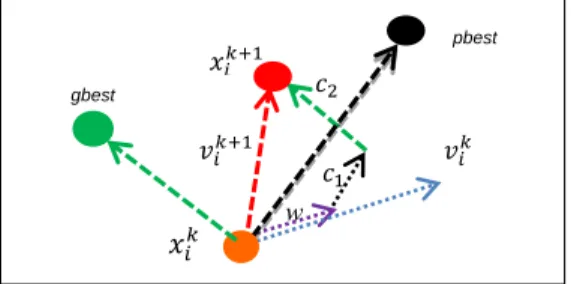
The second step is to update the velocities of all particles at iteration 𝑘 + 1 using the objective or fitness values of particles. The fitness function value of a particle determines which particle has the best global value in the current swarm, 𝑔𝑏𝑒𝑠𝑡 and also determines the best position of each particle over iteration, 𝑝𝑏𝑒𝑠𝑡, The three values that effect the new search direction, namely, current motion, particle own memory, and swarm influence, are incorporated via a summation approach as shown in Eq. (11) with three weight factors, namely, inertia factor, 𝑤, self-confidence factor, 𝑐1, and swarm confidence factor, 𝑐2.
𝑣𝑖𝑘+1= 𝑤 ∙ 𝑣𝑖𝑘+ 𝑐1∙ 𝑟𝑎𝑛𝑑 ∙ (𝑝𝑏𝑒𝑠𝑡 − 𝑥𝑖𝑘) +
𝑐2∙ 𝑟𝑎𝑛𝑑 ∙ (𝑔𝑏𝑒𝑠𝑡 − 𝑥𝑖𝑘) (11)
The appropriate value range for 𝑐1 and 𝑐2 is between 1
and 2, however 2 is the most appropriate in many cases. The following inertia weight is used based on work by Lalitha et al. [10] can be written as
𝑤 = 𝑤𝑚𝑎𝑥− (𝑤𝑚𝑎𝑥− 𝑤𝑚𝑖𝑛)𝑘/𝑘𝑚𝑎𝑥 (12)
where 𝑘𝑚𝑎𝑥, 𝑘 is the maximum number of iterations and
the current number of iterations, respectively. Where, 𝑤𝑚𝑖𝑛 and 𝑤𝑚𝑎𝑥 are the minimum and maximum
weights, respectively. Appropriate values for 𝑤𝑚𝑖𝑛 and
𝑤𝑚𝑎𝑥 are 0.4 and 0.9, respectively proposed by
Eberhart and Shi [11] has been considered in this simulation setup. Position update is the last step in each iteration. The position of each particle is updated using its velocity vector as shown in Eq. (13) and depicted in Figure 4.
𝑥𝑖𝑘+1= 𝑥
𝑖𝑘+ 𝑣𝑖𝑘+1 (13)
The three steps of velocity update, position update, and fitness calculations are repeated until a desired convergence criterion is met.
Figure 4 Velocity and position updates in PSO In the previous section, the PID controller has been designed to control the dynamic parameter of the dynamic robots. The coefficients 𝑘𝑥, 𝑘𝑦 are the
kinematic control parameters and 𝑘𝑢, 𝑘𝑤 are the
velocity control parameters. The PID velocity controller used to maintain the velocities of the mobile robot at desired value as Serrano et al. [12] has experimented it on the PIONEER 3-AT robots. He suggested these values need to be positive to satisfy the stability criteria. In a conventional PID gain tuning method, these parameters are usually selected manually. It is also possible that the parameters are properly chosen, but it cannot be said that the optimal parameters are selected.
To overcome this drawback, this paper adopts the PSO for determining the optimal value of the PID dynamic control parameters. The PSO is utilized off line to determine the gain for the PID controllers. The performance of the controller varies according to adjusted parameters. As aforementioned, each PID block is comprised of one dynamic parameter. Thus, there are, in sum, three control parameters that need to be selected simultaneously for each PID representing the Kp, Ki and Kd. The controller parameters can be written as
w gbest pbest 𝑥𝑖𝑘 𝑣𝑖𝑘+1 𝑥𝑖𝑘+1 𝑣𝑖𝑘 𝑐2 𝒆(𝒕) 𝐾𝑝 𝐾𝑖ʃ 1 𝐾𝑑 𝑑 𝑑𝑡 𝒖(𝒕) 𝑐1 𝑐2
[𝐾𝑝𝑢, 𝐾𝑖𝑢 , 𝐾𝑑𝑢 , 𝐾𝑝𝜔, 𝐾𝑖𝜔 , 𝐾𝑑𝜔], (14)
3.3 The Performance Criteria
In the present study, an integral absolute error (IAE) is utilized to assess the performance of the controller as it is widely adopted to evaluate the dynamic performance of the control system. Based on the calculation by Allaoua et al. [13], the integral of the tracking errors can be calculated as
𝐼𝐴𝐸 = ∫ |𝑒(𝑡)|𝑑𝑡0𝑡 (15)
where 𝑒(𝑡) is the instantaneous error at each iterations. The aim is to minimize this fitness function in order to improve the system response in terms of the steady-state errors. For fitness function calculation, the time-domain simulation of the unicycle mobile robot system model is carried out for the simulation period, 𝑡.
4.0 SIMULATION MODEL
This section discusses the simulation setup for the proposed methodology. In this study, the following
values are used in simulation setup for PID controller parameter optimization [14]:
i. Dimension of the search space = 6 ( i.e., 𝑘𝑖=1…6);
ii. Population/swarm size = 15;
iii. The number of maximum iteration = 100; iv. The self and swarm confident factor, 𝑐1 and 𝑐2
= 2;
v. The inertia weight factor 𝑤 is set by [15], where 𝑤𝑚𝑎𝑥= 0.9 and 𝑤𝑚𝑖𝑛= 0.4;
vi. The searching ranges for the PID gains parameters are limited to (0, 200);
vii. The simulation time, 𝑡 is equal to 250s; viii. Optimization process is repeated 10 times; 4.1 Simulation Platform
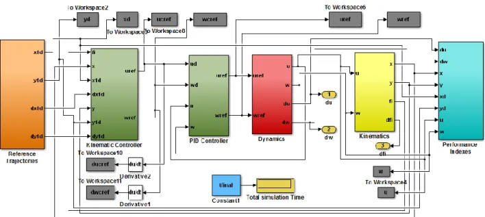
In this section, the corresponding robot kinematic and dynamic parameters as explained in the earlier section are used in the MATLAB-Simulink simulation environment as shown in Figure 5. The PSO algorithm is written in MATLAB mfile.
Figure 5 Simulation modeled using MATLAB-Simulink 4.2 The PID Tuning using PSO
In this section, PSO algorithm is used to optimize parameters of linear and angular velocities controller described in the previous section. The PSO creates a population of 100 swarms that contain the parameters necessary to minimize the objective function. The individuals of the PSO are coded as real values, and the values are shown as below:
[𝐾𝑝𝑢, 𝐾𝑖𝑢 , 𝐾𝑑𝑢 , 𝐾𝑝𝜔, 𝐾𝑖𝜔 , 𝐾𝑑𝜔]= [66.74, 85.23, 53.17,
69.02, 71.75, 53.17]
After applying each best fitness into the PSO-PID velocity controller gains, the whole mobile robot system is simulated by taking into consideration the Pioneer 3-DX complete dynamic model including its speed and acceleration limitations. In this paper, the value for the gains for the kinematic controller, 𝑘𝑥 and
𝑘𝑦 are set as 1.0. Noise was added to the positions and
each simulation was set at 𝑇 = 250𝑠, in which the robot should follow an 8-shape trajectory (varying linear and angular speeds).
5.0 RESULTS AND DISCUSSION
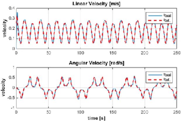
From the simulations, the responses of the linear and velocity controller obtained using the proposed PSO-PID controller is shown in Figure 6. It can be seen that the linear and angular velocities are not much different with those of the reference signals. The rest of the results presented here are categorized into three aspects of verifications; i) smallest fitness function; ii) smaller distance trajectory error and iii) better performance with smaller IAE index.
Figure 6 Linear and angular velocity responses 5.1 Verification 1- Smallest Fitness Function
The objective of utilizing PSO in tuning PID is to get the best optimal gain. The gain value is limited to between 0 and 200. As the number of iterations gets larger, the fitness value becomes smaller. The gain starts to stabilize starting at 50 iterations. The optimal value is reached at fitness 72. Although the iteration is continuing to 100, the fitness value has already reached optimal value at 72 iterations. Figure 7 illustrates this condition. As the MATLAB can capture gain values in each iteration, the one reported here is the fitness value at the point where the fitness is changing, or in other word, in the situation where the PSO found the global best for the two PID gains combination. This changing point is shown in Figure 8. Table 1 shows the fitness values of PID gains at the change points.
Figure 7 Value of the PID gains for the 2 PID block
Figure 8 PID gains tuned using PSO for 100 iterations Table 1 Fitness value of PID gains for velocity controller
No. of
Iteration
Optimal gain parameters Fitness value PID 1 PID 2 2 𝑘𝑝𝑢= 69.19, 𝑘𝑖𝑢= 200.0, 𝑘𝑑𝑢= 149.15, 𝑘𝑝𝜔= 40.27, 𝑘𝑖𝜔= 34.53, 𝑘𝑑𝜔= 200.0, 1.617 4 𝑘𝑝𝑢= 135.05, 𝑘𝑖𝑢= 200.0, 𝑘𝑑𝑢= 140.72, 𝑘𝑝𝜔= 96.92, 𝑘𝑖𝜔= 200.0, 𝑘𝑑𝜔= 200.0, 0.6699 27 𝑘𝑝𝑢= 75.86, 𝑘𝑖𝑢= 199.13, 𝑘𝑑𝑢= 141.05, 𝑘𝑝𝜔= 87.22, 𝑘𝑖𝜔= 147.44, 𝑘𝑑𝜔= 197.56, 0.6658 31 𝑘𝑝𝑢= 106.23, 𝑘𝑖𝑢= 196.27, 𝑘𝑑𝑢= 142.15, 𝑘𝑝𝜔= 58.18, 𝑘𝑖𝜔= 133.25, 𝑘𝑑𝜔= 200.0, 0.5738 45 𝑘𝑝𝑢= 127.47, 𝑘𝑖𝑢= 194.27, 𝑘𝑑𝑢= 142.25, 𝑘𝑝𝜔= 72.18, 𝑘𝑖𝜔= 123.88, 𝑘𝑑𝜔= 200.0, 0.2426 72 𝑘𝑝𝑢= 127.50, 𝑘𝑖𝑢= 194.27, 𝑘𝑑𝑢= 142.25, 𝑘𝑝𝜔= 72.22, 𝑘𝑖𝜔= 123.89, 𝑘𝑑𝜔= 200.0, 0.2128 100 𝑘𝑝𝑢= 127.50, 𝑘𝑖𝑢= 194.27, 𝑘𝑑𝑢= 142.25, 𝑘𝑝𝜔= 72.22, 𝑘𝑖𝜔= 123.89, 𝑘𝑑𝜔= 200.0, 0.2128 𝐾𝑑𝜔 𝐾𝑖𝑢 𝐾𝑑𝑢 𝐾𝑝𝑢 𝐾𝑝𝜔 𝐾𝑖𝜔
5.2 Verification 2- Smaller Distance Trajectory Errors As described in earlier section, the objective of the design of the controller is to reduce the distance error. It is important as it will determine the ability of the controller to ensure the robot position to closely follow a desired trajectory. Figure 9 shows the result for robot trajectory compared with the reference (8-shape), the robot trajectory with GA and robot trajectory run with PSO with 10 iterations. From the graph, it shows that with the PSO-PID controller, the robot has managed to track the reference trajectory with very minimal error compared with GA controller.
The trajectory is related to the distance the robot compared with the reference. As the error is calculated using Eq.5 the result of the distance error is shown in Figure 10. It can be seen that the proposed PSO-PID controller is able to reduce the distance error much better compared with the GA. The distance error can be reduced much better using larger iterations. This can be seen closely in Figure 11.
Figure 9 Robot Trajectory (8-shape reference trajectory) 5.3 Verification 3- Better Performances with Smaller IAE Index
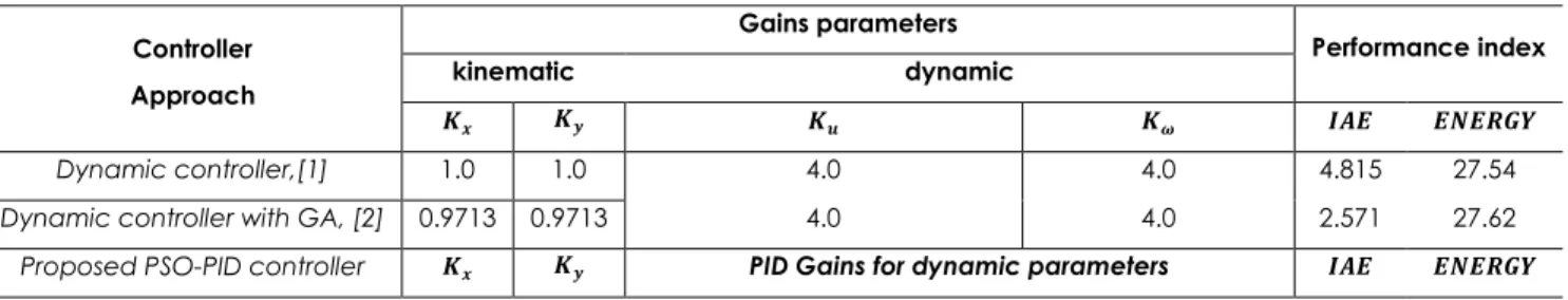
As discussed in the earlier section, the performance criterion is determined based on the IAE and Energy indexes. Some of the resulting PID gains selected by the PSO, associated with the corresponding IAE and
Energy indexes, are shown in Table 2. It can be seen that the smallest IAE value is achieved by the set of bigger gains for dynamic model. It can be seen that the PSO-PID gains also do not consume much energy compared with other approaches, moreover, the PSO-PID controller seems to have smaller IAE index, which indicates stable robot performance.
Figure 10 Distance errors compared using GA and PSO
Figure 11 Distance error with different PSO iteration rate
Table 2 Gain selections associated with the corresponding IAE and energy indexes Controller Approach Gains parameters Performance index kinematic dynamic 𝑲𝒙 𝑲𝒚 𝑲𝒖 𝑲𝝎 𝑰𝑨𝑬 𝑬𝑵𝑬𝑹𝑮𝒀 Dynamic controller,[1] 1.0 1.0 4.0 4.0 4.815 27.54
Dynamic controller with GA, [2] 0.9713 0.9713 4.0 4.0 2.571 27.62 Proposed PSO-PID controller 𝑲𝒙 𝑲𝒚 PID Gains for dynamic parameters 𝑰𝑨𝑬 𝑬𝑵𝑬𝑹𝑮𝒀
𝑲𝒑𝒖 𝑲𝒊𝒖 𝑲𝒅𝒖 𝑲𝒑𝝎 𝑲𝒊𝝎 𝑲𝒅𝝎
PSO-PID 10 iterations 1.0 1.0 190.19 107.22 127.521 52.16 80.03 183.99 1.641 30.15 PSO-PID 20 iterations 1.0 1.0 114.18 39.01 200 97.74 185.29 22.65 1.684 30.02 PSO-PID 100 iterations 1.0 1.0 55.70 51.63 33.28 49.33 65.39 52.89 1.095 29.99
6.0 CONCLUSION
Simulation was performed using MATLAB/Simulink software, employing the dynamic model of the unicycle-like mobile robot presented in section 2 and the PID control structure optimized using PSO proposed in section 3. The presented simulation results show that PSO can be successfully used to select controller gains that result in smaller tracking error and minimizing energy consumption. From the present study, the followings can be concluded:
(a) The two PID controllers optimized with PSO for control the dynamic model of mobile robot is developed.
(b) The validity of the PSO-PID controller is verified with dynamic controller which optimized with GA. (c) The robot trajectory tracking perform better
tracking with smaller distance error compared with the reference trajectory and the robot trajectory with the GA controller.
(d) The performance IAE index is better indicating stable controller performance with nearly same energy consumption.
A limitation of the proposed tuning methods is relies on the accuracy of the robot dynamic model. Therefore, the quality of the tuning results depends on the accuracy of the robot model.
Acknowledgement
The authors express gratitude for the MyBrain15 scholarship from the Malaysian Ministry of Education (MOE) to the first author, and Universiti Teknologi Malaysia for the research facilities.
References
(1) DeVon, D. Bretl, T. 2007. Kinematic and Dynamic Control Of
A Wheeled Mobile Robot. IEEE/RSJ International
Conference on Intelligent Robots and Systems (IROS 2007), San Diego, CA. 29 October 2007. 4065-4070.
(2) Martins, F. N., Celeste, W. C., Carelli, R., Sarcinelli-Filho, M., Bastos-Filho, T. F. 2008. An Adaptive Dynamic Controller For
Autonomous Mobile Robot Trajectory Tracking. Control
Engineering Practice. 16(11): 1354-1363.
(3) Huang, J. T. 2009. Adaptive Tracking Control Of High-Order
Non-Holonomic Mobile Robot Systems. Control Theory and
Applications, IET. 3(6): 681-690.
(4) Oriolo, G., De Luca, A., Vendittelli, M. 2002. WMR Control Via
Dynamic Feedback Linearization: Design, Implementation,
And Experimental Validation. IEEE Transactions on Control
Systems Technology. 10(6): 835-852.
(5) Lee, T. C., Song, K. T., Lee, C. H., Teng, C. C. 2001. Tracking
Control Of Unicycle Modeled Mobile Robots Using A
Saturation Feedback Controller. IEEE Trans. Control System
Technology. 9(2): 305-318.
(6) Martins, F. N., Almeida, G. M., IFES, C. S. 2012. Tuning a
Velocity-based Dynamic Controller for Unicycle Mobile
Robots with Genetic Algorithm. Jornadas Argentinas de
Robotica, JAR. 12: 262-269.
(7) Hassan R, Cohanim B, De Weck O, Venter G. 2005. A
Comparison Of Particle Swarm Optimization And The
Genetic Algorithm. Proceedings of the 1st AIAA
Multidisciplinary Design Optimization Specialist Conference.
Austin, Texas. 18 April 2005. 18-21.
(8) Hashim, N. L. S., Yahya, A., Andromeda, T., Kadir, M. R. R. A.,
Mahmud, N., Samion, S. 2012. Simulation of PSO-PI Controller of DC Motor in Micro--EDM System for Biomedical
Application. Procedia Engineering. 41: 805-811.
(9) De La Cruz, C., Carelli, R. 2006. Dynamic Modeling And
Centralized Formation Control Of Mobile Robots. 32nd
Annual Conference on IEEE Industrial Electronics (IECON), 2006. 6-10 November 2006. Paris. 3880-3885.
(10) Lalitha, M. P., Reddy, V. V., Usha, V. 2010. Optimal DG
Placement For Minimum Real Power Loss In Radial
Distribution Systems Using PSO. Journal of Theoretical and
Applied Information Technology. 13(2): 107-116.
(11) Eberhart, R. C., Shi, Y. 2000. Comparing Inertia Weights And
Constriction Factors In Particle Swarm Optimization. Proceedings of the IEEE Congress on Evolutionary
Computation, La Jolla, CA. 16-19 July 2000. 84-88.
(12) Serrano, M. E., Godoy, S. A., Mut, V. A., Ortiz, O. A. and
Scaglia, G. J. 2015. A Nonlinear Trajectory Tracking Controller For Mobile Robots With Velocity Limitation Via
Parameters Regulation. Robotica. 1-20.
(13) Allaoua, B., Gasbaoui, B., Mebarki, B. 2009. Setting up PID
DC Motor Speed Control Alteration Parameters Using
Particle Swarm Optimization Strategy. Leonardo Electronic
Journal of Practices and Technologies. 14: 19-32.
(14) Basri, M, A., Danapalasingam, K. A., Husain, A. R. 2014.
Design and Optimization of Backstepping Controller for An Underactuated Autonomous Quadrotor Unmanned Aerial
![Figure 1 The differential drive (unicycle-like) mobile robot [2]](https://thumb-us.123doks.com/thumbv2/123dok_us/10945336.2983118/2.918.521.771.88.302/figure-differential-drive-unicycle-like-mobile-robot.webp)