Lecture 15: mixed-effects logistic regression

Lecture 15: mixed-effects logistic regression

28 November 2007

In this lecture we’ll learn about mixed-effects modeling for logistic regres-sion.

1

Technical recap

We moved from generalized linear models (GLMs) to multi-level GLMs by adding a stochastic component to the linear predictor:

η=α+β1X1+· · ·+βnXn+b0+b1Z1+· · ·+bmZm (1)

and usually we assume the random effects vector ~b is normally distributed with mean 0 and variance-covariance matrix Σ.

In a mixed-effects logistic regression model, we simply embed the stochas-tic linear predictor in the binomial error function (recall that in this case, the predicted mean µ corresponds to the binomial parameter p):

P(y;µ) =

n yn

µyn(1−µ)(1−y)n (Binomial error distribution) (2) log µ

1−µ =η (Logit link) (3)

µ= e η

1.1

Fitting multi-level logit models

As with linear mixed models, the likelihood function for a multi-level logit model must marginalize over the random effects ~b:

Lik(β,Σ|~x) =

Z ∞

−∞

P(~x|β, b)P(b|Σ)db (5)

Unfortunately, this likelihood cannot be evaluated exactly and thus the maximum-likelihood solution must be approximated. You can read about some of the approximation methods in Bates (2007, Section 9). Laplacian approximation to ML estimation is available in the lme4 package and is recommended. Penalized quasi-likelihood is also available but not recom-mended, and adaptive Gaussian quadrature is recommended but not yet available.

1.2

An example

We return to thedative dataset and (roughly) follow the example in Baayen Section 7.4. We will construct a model with all the available predictors (except for speaker), and with verb as a random effect. First, however, we need to determine the appropriate scale at which to enter the length (in number of words) of the recipient and theme arguments. Intuitively, both raw scales and log scales are plausible. If our response were continuous, a natural thing to do would be to look at scatterplots of each of these variables against the response. With a binary response, however, such a scatterplot is not very informative. Instead, we take two approaches:

1. Look at the empirical relationship between argument length and mean response, using a shingle;

2. Compare single-variable logistic regressions of response against raw/log argument length and see which version has a better log-likelihood. First we will define convenience functions to use for the first approach:

> tapply.shingle <- function(x,s,fn,...) { result <- c()

x1 <- x[s > l[1] & s < l[2]] result <- c(result, fn(x1,...)) } result } > logit <- function(x) { log(x/(1-x)) }

We then plot the mean response based on shingles (Figure 1):

> my.intervals <- cbind(1:29-0.5,1:29+1.5) > response <- ifelse(dative$RealizationOfRecipient=="PP",1,0) > recipient.x <- with(dative,tapply.shingle(LengthOfRecipient, shingle(LengthOfRecipient,my.intervals),mean)) > recipient.y <- with(dative,tapply.shingle(response, shingle(LengthOfRecipient,my.intervals),mean)) > plot(recipient.x,logit(recipient.y)) > theme.y <- with(dative,tapply.shingle(response, shingle(LengthOfTheme,my.intervals),mean)) > theme.x <- with(dative,tapply.shingle(LengthOfTheme, shingle(LengthOfTheme,my.intervals),mean)) > plot(theme.x,logit(theme.y))

These plots are somewhat ambiguous and could support either a linear or logarithmic relationship in logit space. (Keep in mind that (a) we’re not seeing points where there are 100% of responses that are “successful” or “failures”; and (b) there are very few data points at the larger lengths.) So we resort to the logistic regression approach (recall that the deviance is simply -2 times the log-likelihood):

> summary(glm(response ~ LengthOfTheme,dative, family="binomial"))$deviance [1] 3583.41 > summary(glm(response ~ log(LengthOfTheme),dative, family="binomial"))$deviance [1] 3537.279 > summary(glm(response ~ LengthOfRecipient,dative,

Figure 1: Responses of recipient and theme based on shingles family="binomial"))$deviance [1] 3104.92 > summary(glm(response ~ log(LengthOfRecipient),dative, family="binomial"))$deviance [1] 2979.884

In both cases the log-length regression has a lower deviance and hence a higher log-likelihood. So we’ll enter these terms into the overall mixed-effects regression as log-lengths. > dative.glmm <- lmer(RealizationOfRecipient ~ log(LengthOfRecipient) + log(LengthOfTheme) + AnimacyOfRec + AnimacyOfTheme + AccessOfRec + AccessOfTheme + PronomOfRec + PronomOfTheme + DefinOfRec + DefinOfTheme + SemanticClass +

Modality + (1 | Verb), dative,family="binomial",method="Laplace") > dative.glmm

[...]

Groups Name Variance Std.Dev. Verb (Intercept) 4.6872 2.165 number of obs: 3263, groups: Verb, 75

Estimated scale (compare to 1 ) 0.7931773 Fixed effects:

Estimate Std. Error z value Pr(>|z|) (Intercept) 1.9463 0.6899 2.821 0.004787 ** AccessOfThemegiven 1.6266 0.2764 5.886 3.97e-09 *** AccessOfThemenew -0.3957 0.1950 -2.029 0.042451 * AccessOfRecgiven -1.2402 0.2264 -5.479 4.28e-08 *** AccessOfRecnew 0.2753 0.2472 1.113 0.265528 log(LengthOfRecipient) 1.2891 0.1552 8.306 < 2e-16 *** log(LengthOfTheme) -1.1425 0.1100 -10.390 < 2e-16 *** AnimacyOfRecinanimate 2.1889 0.2695 8.123 4.53e-16 *** AnimacyOfThemeinanimate -0.8875 0.4991 -1.778 0.075334 . PronomOfRecpronominal -1.5576 0.2491 -6.253 4.02e-10 *** PronomOfThemepronominal 2.1450 0.2654 8.081 6.40e-16 *** DefinOfRecindefinite 0.7890 0.2087 3.780 0.000157 *** DefinOfThemeindefinite -1.0703 0.1990 -5.379 7.49e-08 *** SemanticClassc 0.4001 0.3744 1.069 0.285294 SemanticClassf 0.1435 0.6152 0.233 0.815584 SemanticClassp -4.1015 1.5371 -2.668 0.007624 ** SemanticClasst 0.2526 0.2137 1.182 0.237151 Modalitywritten 0.1307 0.2096 0.623 0.533008

(Incidentally, this model has higher log-likelihood than the same model with raw instead of log- argument length, supporting our choice of log-length as the preferred predictor.)

The fixed-effect coefficients can be interpreted as normal in a logistic regression. It is important to note that there is considerable variance in the random effect of verb. The scale of the random effect is that of the linear predictor, and if we consult the logistic curve we can see that a standard deviation of 2.165 means that it would be quite typical for the magnitude of this random effect to be the difference between a PO response probability of 0.1 and 0.5.

Figure 2: Random intercept for each verb in analysis of the dative dataset Because of this considerable variance of the effect of verb, it is worth looking at the BLUPs for the random verb intercept:

> nms <- rownames(ranef(dative.glmm)$Verb) > intercepts <- ranef(dative.glmm)$Verb[,1]

> support <- tapply(dative$Verb,dative$Verb,length) > labels <- paste(nms,support)

> barplot(intercepts[order(intercepts)],names.arg=labels[order(intercepts)], las=3,mgp=c(3,-0.5,0),ylim=c(-6,4)) # mgp fix to give room for verb names

The results are shown in Figure 2. On the labels axis, each verb is followed by its support: the number of instances in which it appears in the dative

dataset. Verbs with larger support will have more reliable random-intercept BLUPs. From the barplot we can see that verbs including tell, teach, and show are strongly biased toward the double-object construction, whereas send,bring,sell, andtake are strongly biased toward the prepositional-object construction.

This result is theoretically interesting because the dative alternation has been at the crux of a multifaceted debate that includes:

• whether the alternation is meaning-invariant;

• if it is not meaning-invariant, whether the alternants are best handled via constructional or lexicalist models;

• whether verb-specific preferences observable in terms of raw frequency truly have their locus at the verb, or can be explained away by other properties of the individual clauses at issue.

Because verb-specific preferences in this model play such a strong role de-spite the fact that many other factors are controlled for, we are on better footing to reject the alternative raised by the third bullet above that verb-specific preferences can be entirely explained away by other properties of the individual clauses. Of course, it is always possible that there are other ex-planatory factors correlated with verb identity that will completely explain away verb-specific preferences; but this is the nature of science. (This is also a situation where controlled, designed experiments can play an important role by eliminating the correlations between predictors.)

1.3

Model comparison & hypothesis testing

For nested mixed-effects logit models differing only in fixed-effects structure, likelihood-ratio tests can be used for model comparison. Likelihood-ratio tests are especially useful for assessing the significance of predictors consisting of factors with more than two levels, because such a predictor simultaneously introduces more than one parameter in the model:

> dative.glmm.noacc <- lmer(RealizationOfRecipient ~ log(LengthOfRecipient) + log(LengthOfTheme) + AnimacyOfRec + AnimacyOfTheme + PronomOfRec + PronomOfTheme + DefinOfRec + DefinOfTheme + SemanticClass +

Modality + (1 | Verb), dative,family="binomial",method="Laplace") > anova(dative.glmm,dative.glmm.noaccessibility)

[...]

Df AIC BIC logLik Chisq Chi Df Pr(>Chisq) dative.glmm.noacc 15 1543.96 1635.31 -756.98 dative.glmm 19 1470.93 1586.65 -716.46 81.027 4 < 2.2e-16 *** > dative.glmm.nosem <- lmer(RealizationOfRecipient ~ log(LengthOfRecipient) + log(LengthOfTheme) + AnimacyOfRec + AnimacyOfTheme + AccessOfRec + AccessOfTheme + PronomOfRec + PronomOfTheme + DefinOfRec + DefinOfTheme +

Modality + (1 | Verb), dative,family="binomial",method="Laplace") > anova(dative.glmm,dative.glmm.nosem)

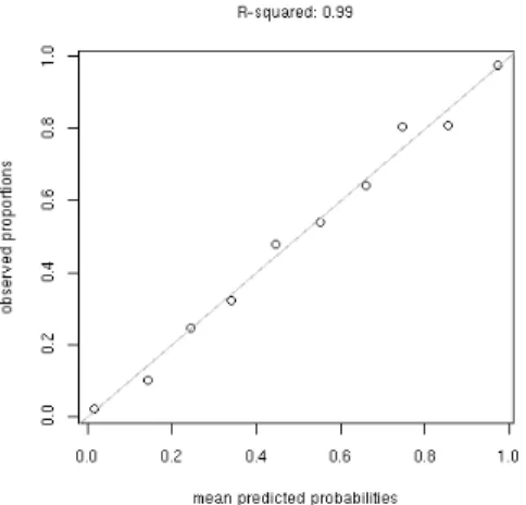
Figure 3: The fit between predicted and observed probabilities for each decile of predicted probability for dative.glmm

[...]

Df AIC BIC logLik Chisq Chi Df Pr(>Chisq) dative.glmm.nosem 15 1474.55 1565.90 -722.27

dative.glmm 19 1470.93 1586.65 -716.46 11.618 4 0.02043 *

1.4

Assessing a logit model

When assessing the fit of a model whose response is continuous, a plot of the residuals is always useful. This is not a sensible strategy for assessing the fit of a model whose response is categorical. Something that is often done instead is to plot predicted probability against observed proportion for some binning of the data. This process is described in Baayen page 305, through the languageRfunction plot.logistic.fit.fnc():

> plot.logistic.fit.fnc(dative.glmm,dative)

This is really a very good fit.

Finally, a slight word of warning: our model assumed that the random verb-specific intercepts are normally distributed. As a sanity check, we can use the Shapiro-Wilk test to check the distribution of BLUPs for the intercepts:

> shapiro.test(ranef(dative.glmm)$Verb[,1]) Shapiro-Wilk normality test

data: intercepts

W = 0.9584, p-value = 0.0148

There is some evidence here that the intercepts are not normally distributed. This is more alarming given that the model has assumed that the intercepts are normally distributed, so that it is biased toward assigning BLUPs that adhere to a normal distribution.

2

Further Reading

There is good theoretical coverage (and some examples) of GLMMs in Agresti (2002, Chapter 12). There is a bit of R-specific coverage in Venables and Ripley (2002, Section 10.4) which is useful to read as a set of applie examples, but the code they present uses penalized quasi-likelihood estimation and this is outdated by lme4.

References

Agresti, A. (2002). Categorical Data Analysis. Wiley, second edition.

Bates, D. (2007). Linear mixed model implementation in lme4. Manuscript, University of Wisconsin, 15 May 2007.

Venables, W. N. and Ripley, B. D. (2002). Modern Applied Statistics with S. Springer, fourth edition.