Accelerating Radiation Dose Calculation with High Performance Computing and Machine Learning for Large-scale Radiotherapy Treatment Planning

UCLA

UCLA Electronic Theses and Dissertations

Accelerating Radiation Dose Calculation with High Performance Computing and Machine Learning for Large-scale Radiotherapy Treatment Planning

Permalink https://escholarship.org/uc/item/2np1b05w Author Neph, Ryan Publication Date 2020 Peer reviewed|Thesis/dissertation

UNIVERSITY OF CALIFORNIA Los Angeles

Accelerating Radiation Dose Calculation with High Performance Computing and Machine Learning for Large-scale Radiotherapy Treatment Planning

A dissertation submitted in partial satisfaction of the requirements for the degree Doctor of Philosophy

in Physics and Biology in Medicine

by

Ryan Thomas Neph

© Copyright by Ryan Thomas Neph

ABSTRACT OF THE DISSERTATION

Accelerating Radiation Dose Calculation with High Performance Computing and Machine Learning for Large-scale Radiotherapy Treatment Planning

by

Ryan Thomas Neph

Doctor of Philosophy in Physics and Biology in Medicine University of California, Los Angeles, 2020

Professor Ke Sheng, Chair

Radiation therapy is powered by modern techniques in precise planning and execution of radiation delivery, which are being rapidly improved to maximize its benefit to cancer patients. In the last decade, radiotherapy experienced the introduction of advanced methods for automatic beam orientation optimization, real-time tumor tracking, daily plan adaptation, and many others, which improve the radiation delivery precision, planning ease and reproducibility, and treatment efficacy. However, such advanced paradigms necessitate the calculation of orders of magnitude more causal dose deposition data, increasing the time requirement of all pre-planning dose calculation. Principles of high-performance computing and machine learning were applied to address the insufficient speeds of widely-used dose calculation algorithms to facilitate translation of these advanced treatment paradigms into

To accelerate CT-guided X-ray therapies, Collapsed-Cone Convolution-Superposition (CCCS), a state-of-the-art analytical dose calculation algorithm, was accelerated through its novel implementation on highly parallelized GPUs. This context-based GPU-CCCS approach takes advantage of X-ray dose deposition compactness to parallelize calculation across hundreds of beamlets, reducing hardware-specific overheads, and enabling acceleration by two to three orders of magnitude compared to existing GPU-based beamlet-by-beamlet approaches. Near-linear increases in acceleration are achieved with a distributed, multi-GPU implementation of context-based GPU-CCCS.

Dose calculation for MR-guided treatment is complicated by electron return effects (EREs), exhibited by ionizing electrons in the strong magnetic field of the MRI scanner. EREs necessitate the use of much slower Monte Carlo (MC) dose calculation, limiting the clinical application of advanced treatment paradigms due to time restrictions. An automatically distributed framework for very-large-scale MC dose calculation was developed, granting linear scaling of dose calculation speed with the number of utilized computational cores. It was then harnessed to efficiently generate a large dataset of paired high- and low-noise MC doses in a 1.5 tesla magnetic field, which were used to train a novel deep convolutional neural network (CNN), DeepMC, to predict low-noise dose from faster high-noise MC-simulation. DeepMC enables 38-fold acceleration of MR-guided X-ray beamlet dose calculation, while remaining synergistic with existing MC acceleration techniques to achieve multiplicative speed improvements.

This work redefines the expectation of X-ray dose calculation speed, making it possible to apply new highly-beneficial treatment paradigms to standard clinical practice for the first time.

The dissertation of Ryan Thomas Neph is approved. Dan Ruan James Michael Lamb

Xun Jia You Ming Yang Ke Sheng, Committee Chair

University of California, Los Angeles 2020

TABLE OF CONTENTS

List of Tables ... x

List of Figures ... xi

List of Equations ... xvi

Acknowledgements ... xvii

Vita ... xix

1 INTRODUCTION ... 1

2 OVERVIEW OF RADIATION THERAPY ... 3

2.1 Radiation Dose Deposition Mechanisms... 3

2.1.1 Electromagnetic Radiation ... 5

2.1.1.1 The Photoelectric Effect ... 5

2.1.1.2 The Compton Effect... 6

2.1.1.3 Pair Production ... 7

2.1.2 Particulate Radiation ... 8

2.1.2.1 Electrons ... 10

2.1.2.2 Protons and Heavy Ions ... 10

2.1.2.3 Electromagnetic Field Effects... 11

2.2 Dose Calculation Algorithms ... 12

2.2.1 Monte Carlo Dose Calculation ... 13

2.2.2 Analytical Dose Calculation ... 14

2.2.3 Linearized Boltzmann Solvers ... 15

2.3 Radiation Treatment Planning... 16

2.3.1 Beamlet Dose Calculation ... 17

2.3.2 Inverse Treatment Planning ... 18

2.3.3 Final Dose Calculation ... 19

2.3.4 Online Adaptive Radiotherapy ... 20

3 PARALLEL BEAMLET DOSE CALCULATION VIA BEAMLET CONTEXTS IN A DISTRIBUTED MULTI-GPU FRAMEWORK34 _{... 21}

3.2.1 Nonvoxel-Based Dose Calculation ... 25

3.2.1.1 Beamlet-based Dose by Intra-beam Parallelization ... 25

3.2.1.1.1 TERMA Calculation ... 25

3.2.1.1.2 Beamlet Context Extraction ... 28

3.2.1.1.3 Nonvoxel-Based Transformation ... 32

3.2.1.1.4 Dose Ray Convolution ... 34

3.2.1.1.5 Beamlet Context Dose Extraction ... 35

3.2.1.2 Distributed Parallelization ... 35

3.2.2 Measuring Computational Efficiency... 36

3.2.3 Measuring Dosimetric Accuracy ... 37

3.3 Results ... 40

3.4 Discussion ... 46

3.4.1 Performance ... 46

3.4.2 Accuracy ... 50

3.5 Applications ... 53

3.5.1 A sparse orthogonal collimator for small animal intensity‐modulated radiation therapy79,80 _{... 54}

3.5.1.1 Background ... 54

3.5.1.2 Methods ... 55

3.5.1.3 Results and Discussion ... 58

3.5.2 A novel optimization framework for VMAT with dynamic gantry couch rotation40 _{... 61}

3.5.2.1 Background ... 61

3.5.2.2 Methods ... 62

3.5.2.3 Results and Conclusions... 64

3.5.3 Single-Arc VMAT optimization for Dual-Layer MLC44 _{... 65}

3.5.3.1 Background ... 65

3.5.3.2 Methods ... 65

3.5.3.3 Results and Conclusions... 67

3.5.4.1 Background ... 69

3.5.4.2 Methods ... 70

3.5.4.3 Results and Conclusions... 72

3.6 Conclusions ... 74

4 A HIGH-PERFORMANCE DISTRIBUTED FRAMEWORK FOR LARGE-SCALE MONTE CARLO DOSE CALCULATION ... 76

4.1 Introduction ... 76

4.2 Implementation ... 78

4.2.1 Distributed Computation Model ... 78

4.2.2 Orchestration and Scalability ... 83

4.2.3 SimpleDose: A High-Level Treatment Planning Interface ... 84

4.3 Usage Examples ... 85

4.4 Performance ... 88

4.5 Conclusions ... 89

5 DEEPMC: A DEEP LEARNING METHOD FOR EFFICIENT MONTE CARLO BEAMLET DOSE CALCULATION BY PREDICTIVE DENOISING IN MAGNETIC RESONANCE-GUIDED RADIOTHERAPY ... 90

5.1 Introduction ... 90

5.2 Preliminary Investigation in Stacked Slab Phantom Geometries ... 93

5.3 Methods ... 96

5.3.1 DeepMC Model Architecture ... 96

5.3.2 Dose Data Generation ... 100

5.3.3 Experiment Design ... 103

5.4 Results ... 106

5.5 Discussion ... 112

5.6 Conclusions ... 114

5.7 Appendices ... 116

5.7.1 Appendix A. Dose Volume Histograms ... 116

5.7.4 Appendix D. Fluence Map Comparison ... 119

6 SUMMARY OF WORK ... 120 7 REFERENCES ... 123

L

IST OF

T

ABLES

Table 3-1. Per-beam Calculation Times (average, in seconds) ...41 Table 3-2. Peak Memory Usage For GPU-based CCCS Methods (in Megabytes) ...43 Table 3-3. Comparisons between the measured and intended dose distributions for the C-shaped target plan and the mouse phantom whole liver plan. Table reproduced from Woods et al. (2019)80_{. ...58}

Table 3-4. Number of feasible beams, prescription doses and PTV volumes for all patients. Table reproduced from Lyu et al. (2020)43_{. ...71}

Table 5-1. Plan quality metrics derived from deliverable dose to the first testing patient for plans optimized using different beamlet dose calculation methods. ... 108 Table 5-B1. Plan quality metrics derived from deliverable dose to the second testing patient

L

IST OF

F

IGURES

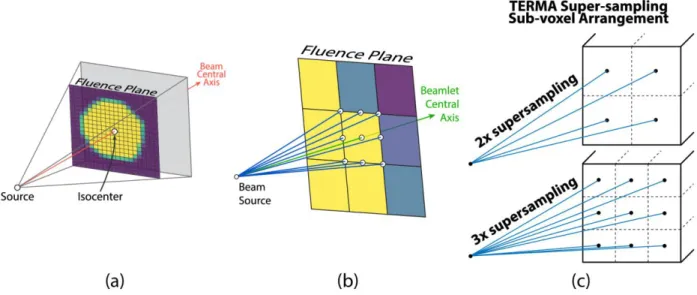
Figure 3-1. (a) Intersection map for one beam orientation and target volume definition. Purple-colored cells have no target intersection and are excluded from beamlet-dose calculation, yellow: full intersection, others: partial intersection. (b) Super-sampling ray layout for testing beamlet-target intersection. (c) cross-section of TERMA calculation sub-voxel arrangement for super-sampled averaging (2x and 3x options shown for one voxel). ...26 Figure 3-2. (a) Beamlet dose calculation workflow. A single worker node processes beams in

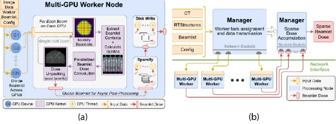
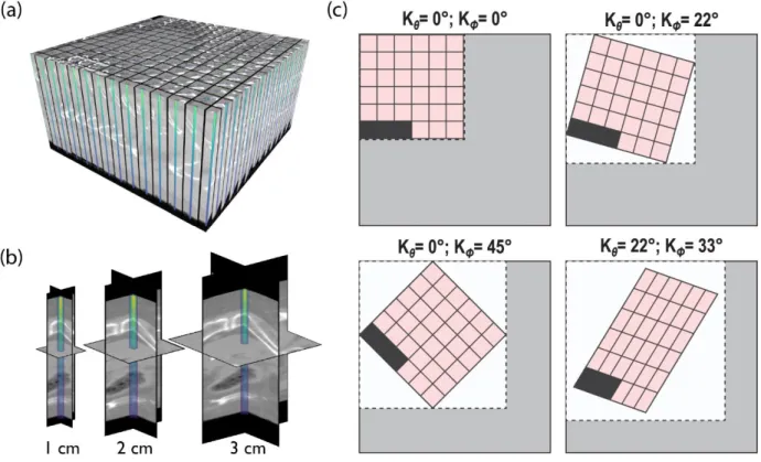
parallel across its resident GPU devices. Beamlet processing is further parallelized on a GPU using beamlet contexts. (b) Distributed computing framework. The manager node prepares independent task lists for each worker node to process in parallel and receives the results for delivery to the requestor. ...28 Figure 3-3. (a) Visualization of the beamlet context array for a single beam including

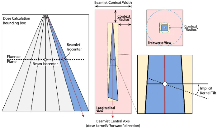
contextual densities and beamlet-specific dose after calculation. (b) Beamlet context cross sections for various context radii with dose overlaid. (c) Convolution-ray-aligned context array (cross-section) for various kernel rays. Grey area is allocated once and reused for all beams. White subregions are allotted for kernel-ray-specific convolutions geometry. Black cells indicate unused space after packing beamlet contexts into the array. Convolution direction is into page. ...31 Figure 3-4. Construction of one beamlet context with implicit kernel tilting. Blue region

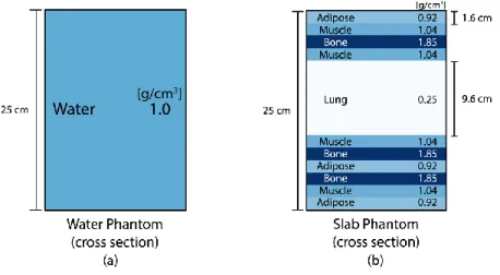
indicates the volume of non-zero TERMA for a single beamlet. The distance between the blue rings in the transverse view is representative of the context radius setting. The union of red and gold boxes represents the volume in which dose is computed. ...32 Figure 3-5. Cross sections of phantom geometries with beam entering from the top; used to

assess dosimetric accuracy. Materials and densities are provided. ...38 Figure 3-6. Performance for single-node and multi-node scaling strategies. For multi-node

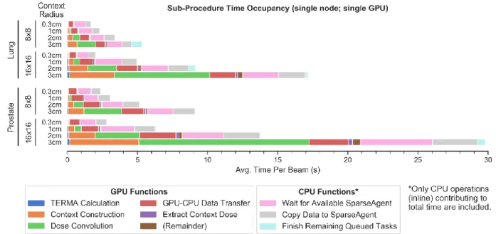
measurements, each node was configured with 2 GPUs. The dotted black line indicates theoretical linear scaling in multi-node setups. ...41 Figure 3-7. Fractional execution time spent in each sub-procedure on one computational

node with 4 threaded post-processing “SparseAgents”. Only time spent on the main

processing thread is represented. ...42 Figure 3-8. Fractional execution time for 1cm context radius with a variable number of

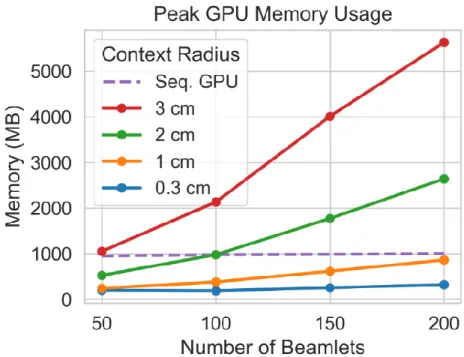
background post-processing (dose sparsification) threads. Only time spent on the main processing thread is represented. ...42 Figure 3-9. Peak memory usage for various beamlet counts and context radii. ...43

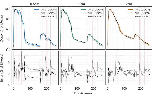
Figure 3-10. Single-beamlet depth dose and lateral profiles in the water phantom for increasing beamlet widths. Error is calculated between our context-based GPU-CCCS method and each of CPU-CCCS and Monte Carlo. ...44 Figure 3-11. Single-beamlet depth dose and lateral profiles in the stack of slabs phantom for

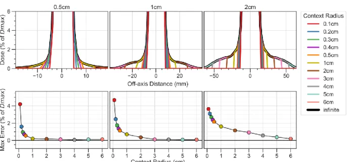
increasing beamlet widths. Error is calculated between our context-based GPU-CCCS method and each of CPU-CCCS and Monte Carlo. ...45 Figure 3-12. Central lateral line profile in the water phantom at 10cm depth for various

beamlet widths and context radii pairs (top). Maximum errors (%) between non-context-based (infinite radius) and non-context-based dose profiles are provided (bottom). The dose is normalized to the maximum dose in the volume. Y-axis range is limited to better depict low dose beamlet penumbra region where context-based approximation is active. ...46 Figure 3-13. Lateral line profile in the water phantom at various depths for a 5×5cm2 _broad

beam calculated as the sum of 5×5mm2 _{beamlets for various context radii at three} depths. Dose for “infinite” radius was computed without context-based approximation. ...53 Figure 3-14. (Left) Mouse phantom modeled from mouse CT data and 3D-printed with a

flexible, tissue-equivalent material and a mid-coronal split for film measurement. Phantom is shown on the previously mentioned rotating couch mount. (Right) 3D-printed block phantom for axial dose measurements. Figure reproduced from Woods et al. (2019)80_{. ...57}

Figure 3-15. (Left) Calculated dose distribution of the C-shaped target plan perpendicular to the gantry rotation axis. (Center) Measured film dose distribution from the center of the solid water phantom for the C target plan delivered with the SOC. Both plans are shown with the same color scale, in units of Gy. (Right) A comparison of the calculated (yellow) and measured (blue) 50% isodose lines, with overlapping regions shown in red. Figure reproduced from Woods et al. (2019)80_{. ...58}

Figure 3-16. (A) Mid-coronal view of the calculated dose for the mouse phantom whole liver plan (units of Gy). (B) The 5 optimal coplanar beam angles selected with the 4π

algorithm. (C) Measured film dose from the mouse phantom, treated with the whole liver plan, at the plane shown in A (units of Gy). (D) A comparison of the calculated (yellow) and measured (blue) 60% isodose lines, with overlapping regions shown in red. *Target structure was rotated to account for slight phantom misalignment, which also resulted in the truncated lower left portion of the target. Figure reproduced from Woods et al. (2019)80_{. ...60}

the SOC. Both plans are shown with the same color scale, in units of Gy. Figure reproduced from Woods et al. (2019)80_{. ...61}

Figure 3-18. Demonstration of (A) DLMLC with 10mm leaf width (DLMLC-10mm), (B) SLMLC with 5mm leaf width (SLMLC-5mm), (C) SLMLC with 10mm leaf width (SLMLC-10mm), (D) SLMLC with 10mm leaf width and 5mm leaf step size (SLMLC-10mm-5mm). The grids on (C) and (D) represent the achievable beamlets. Figure reproduced from Lyu et al. (2019)44_{. ...66}

Figure 3-19. DVH for (A) the GBM case, (B) the LNG case, (C) the PRT case, and (D) the REC-SIB case. The solid lines are for the DLMLC plan, and the dotted lines are for SLMLC plans. D95 is normalized to the prescription dose. Figure reproduced from Lyu et al.

(2019)44_{. ...69}

Figure 3-20. (A) Demonstration of the robotic arm platform, (B) an isocentric SID-100 beam that covers the entire target, (C) beams of different isocenters are required to efficiently cover the entire target. Figure reproduced from Lyu et al. (2020)43_{. ...70}

Figure 3-21. Final objective value vs the number of beams. The plot with shaded error bar shows a summary of all patients. Each patient plot is titled with the patient number, the number of isocenters for the SID-50 plan, and the number of isocenters for the SID-100

plan. For example, the first patient plot is entitled: ‘#1: 4(50), 1(100)’, showing that the

patient #1 has four isocenters for the SID-50 plan, and one isocenter for the SID-100 plan. Figure reproduced from Lyu et al. (2020)43_{. ...73}

Figure 4-1. Database document hierarchy. Simulations are organized as children of a sub-beam (sub-beamlet or spot). Sub-sub-beams are children of a sub-beam. Multiple sub-beams can be defined for a single calculation geometry and multiple geometries can be defined for a CT image acquisition. Images contain masks for every structure defined in the RTStruct file. Simulations can produce one or more independent samples of dose for the same configuration as a method for machine learning dataset augmentation. ...81 Figure 4-2. Summary of commands available from the SimpleDose interface for treatment

planning dose calculation. ...85 Figure 4-3. Create-plan command output using the SimpleDose to add dose calculation

requests for automatically distributed computation. ...86 Figure 4-4. Plan-status command output using the SimpleDose interface to list the simulation

progress for all existing plans. ...87 Figure 4-5. Sparse storage format for calculated planning dose results for a SimpleDose plan.

The sparse coordinate list (COO) format uses three equal-length arrays to store the row index, column index, and data value for every non-zero element of the represented matrix. ...88

Figure 5-1. Slab phantom geometry specification for studying electron return effects present at high-density-gradient tissue interfaces. ...94 Figure 5-2. MC dose ground truth (low-noise.), model input (high-noise) and DeepMCv1

prediction for a photon beamlet in the low dose penumbra region (1.25cm off-axis) of water/air (left) and aluminum/air (right) slab phantoms. Lines indicate positions of horizontal material interfaces. Low-noise dose was simulated using 18M particles in ~3 minutes. High-noise dose was simulated using 30K particles in 3 seconds. Prediction took <100ms after high-noise dose simulation. ...95 Figure 5-3. Fully convolutional model architecture used by our method, DeepMC. Numbers

in blocks indicate number of feature channels produced by learned convolutional kernels at each stage. 3×3×3 kernels are used in UNet layers. 1×1×1 kernels are used

for feature mixing and dose prediction. ...98 Figure 5-4. DeepMC training progress. Per-epoch loss is shown for training dataset (grey)

and validation dataset (orange). ...98 Figure 5-5. Dose from low- and high-noise MC simulation and DeepMC prediction for one

5x5mm2 _{x-ray beamlet. Three adjacent slices are shown with their transverse distance} from the beamlet’s central axis listed in the titles. Color scale limits are displayed in the

lower left corner for each slice in normalized units. Arrows show examples of electron return effects asymmetrically perturbing the dose deposition. High-noise simulation fails to accurately estimate dose in these areas while DeepMC dose matches the low-noise ground truth dose. ...99 Figure 5-6. Observed density (left) and cumulative density (right) of voxelized x-ray dose,

normalized to per-beamlet maxima. Voxels with dose lower than 10% of per-beamlet maxima account for over 99% of observations. Vertical axes are displayed in log-scale. ...99 Figure 5-7. Dose volume histogram comparing “deliverable” dose for IMRT treatment plans

created using low-noise ground truth, DeepMC-predicted, and high-noise beamlet dose for testing patient one (left) and two (right). Doses for all plans are recalculated after plan optimization using low-noise beamlet dose to reflect the deliverable dose to each patient. ... 107 Figure 5-8. Deliverable dose color washes for axial slices from the first testing patient.

Deliverable dose for each plan is recalculated using low-noise beamlet dose after plan optimization. The last two columns show differences in deliverable dose attributed to using either high-noise or DeepMC-predicted dose approximations to optimize IMRT beamlet fluence. Colors scales are consistent for each row; scale limits shown on the color bar in absolute dose units of Gy. ... 110

Figure 5-9. Planning and deliverable dose color washes for axial slices from the first testing patient. Planning dose is used directly for plan optimization. Deliverable dose for each plan is recalculated using low-noise beamlet dose after plan optimization. The Last two columns show differences in planning and deliverable dose for each plan. Color scales are consistent for each row; scale limits shown on the color bar are in absolute dose units of Gy. ... 111 Figure 5-10. Plan delivery parameters (X-ray beamlet fluence) for the first testing patient

resulting from optimization using DeepMC, high-, and low-noise beamlet dose. All color scales are consistent, and limits are shown in the color bars on the right. All are normalized to the per-beam maximum fluence from the ground truth plan. ... 111 Figures 5-A1 through 5-A4. Dose volume histograms for treatment plans created using

DeepMC-predicted (top) and high-noise MC-simulated (bottom) beamlet dose. Ground truth plans are created using low-noise MC-simulated dose. Dose for “planning” curves is calculated using each plan’s respective beamlet dose after plan optimization. Dose for “deliverable” curves is recalculated using low-noise dose for more accurate, but more computationally expensive plan quality evaluation. ... 116 Figure 5-C1. Deliverable dose washes for axial slices from the second testing patient. Deliverable dose for each plan is recalculated using low-noise beamlet dose after plan optimization. The last two columns show differences in deliverable dose attributed to using either high-noise or DeepMC-predicted dose approximations to optimize IMRT beamlet fluence. Colors scales are consistent for each row; scale limits shown on the color bar in absolute dose units of Gy. ... 117 Figure 5-C2. Planning and deliverable dose color washes for axial slices from the second testing patient. Planning dose is used directly for plan optimization. Deliverable dose for each plan is recalculated using low-noise beamlet dose after plan optimization. The Last two columns show differences in planning and deliverable dose for each plan. Color scales are consistent for each row; scale limits shown on the color bar are in absolute dose units of Gy. ... 118 Figure 5-D1. Plan delivery parameters (X-ray beamlet fluence) for the second testing patient one resulting from optimization using DeepMC, high-, and low-noise ground truth beamlet dose. All color scales are matched consistent, and limits are shown in the color bars on the right. All are normalized to the per-beam ground truth maximum fluence from the ground truth plan. ... 119

L

IST OF

E

QUATIONS

A

CKNOWLEDGEMENTS

For his incredible support over these years, I’d like to thank my advisor Dr. Ke Sheng, who gave me the stability and encouragement to pursue research in the topics of machine learning and high performance computing that were of great interest to me. I am extremely grateful for the mentorship provided by Ke and his many collaborators, particularly Dr. Dan Ruan and Dr. Youming Yang for lending a critical mind to improve the quality of my work and help steer me in the right direction.

I’d also like to thank all of the UCLA Physics in Biology in Medicine faculty and staff for devoting their efforts to educate my fellow students and me in the principles and practices of Medical Physics, and make our graduate school experience enjoyable and memorable. I am lucky to have made such great friends as I have in my research lab, and in the PBM program at UCLA. Thank you to Dan, Victoria, Angelia, Kaley, Daniel, Wenbo, Qihui, Elizabeth, Daili, Jiayi, Pav, Ningning, Yang, Nuo, Lingli, Yi, and Alan for your camaraderie in the trenches of scientific research. Thanks also to Geri, John, Kamal, Nastaran, Jason, Ksenia, and Wenbo for the lasting friendship that all began when we arrived for orientation in the fall of 2015. Special thanks to my parents for raising me and encouraging me to seek out answers to the questions of the world, my sister for walking ahead of me on the path to higher education, my uncle John for exposing me to science and technology at an early age and fostering my process of logical reasoning. I’d especially like to thank my wife Ashley for tolerating the many challenges of raising two children with me in Los Angeles on a single graduate

my academic goals. I could not have accomplished all I have without each and every one of you, and I will be forever in your debt.

Section 3.8.1 is a shortened version of:

Woods, K., Nguyen, D., Neph, R., Ruan, D., O’Connor, D., & Sheng, K. (2019). A sparse orthogonal collimator for small animal intensity‐modulated radiation therapy part I:

Planning system development and commissioning. Medical Physics, 46(12), 5703–

5713. https://doi.org/10.1002/mp.13872

and Woods, K., Neph, R., Nguyen, D., & Sheng, K. (2019). A sparse orthogonal collimator

for small animal intensity‐modulated radiation therapy. Part II: hardware

development and commissioning. Medical Physics, 46(12), 5733–5747. https://doi.org/10.1002/mp.13870.

Section 3.8.2 is a shortened version of:

Lyu, Q., Yu, V. Y., Ruan, D., Neph, R., O’Connor, D., & Sheng, K. (2018). A novel optimization

framework for VMAT with dynamic gantry couch rotation. Physics in Medicine & Biology, 63(12), 125013. https://doi.org/10.1088/1361-6560/aac704.

Section 3.8.3 is a shortened version of:

Lyu, Q., Neph, R., Yu, V. Y., Ruan, D., & Sheng, K. (2019). Single-arc VMAT optimization for dual-layer MLC. Physics in Medicine & Biology, 64(9), 095028. https://doi.org/10.1088/1361-6560/ab0ddd.

Section 3.8.4 is a shortened version of:

Lyu, Q., Neph, R., Yu, V. Y., Ruan, D., Boucher, S., & Sheng, K. (2020). Many-isocenter optimization for robotic radiotherapy. Physics in Medicine and Biology, 65(4). https://doi.org/10.1088/1361-6560/ab63b8.

Chapter 3 is a version of a published journal article:

Neph R, Ouyang C, Neylon J, Yang YM, Sheng K. Parallel beamlet dose calculation via beamlet contexts in a distributed multi‐GPU framework. Med Phys. June 2019:mp.13651. doi:10.1002/mp.13651.

Chapter 5 is a version of a manuscript currently under review for publication:

Neph R, Lyu Q, Huang Y, Yang YM, Sheng K. DeepMC: a deep learning method for efficient monte carlo beamlet dose calculation by predictive denoising in magnetic

resonance-V

ITA

EDUCATION

M.S. University of California, Los Angeles, Physics and Biology in Medicine 2019 B.S. Kettering University, Engineering Physics 2015 B.S. Kettering University, Mechanical Engineering 2015

AWARDS

Norm Baily Award 1st _{place prize (AAPM Southern California Chapter) 2019}

Science Council’s Scientific Session - Selected Speaker (AAPM Annual Meeting) 2019 Best Poster (UCLA Physics and Biology in Medicine Research Colloquium) 2017

PEER-REVIEWED PUBLICATIONS

Shang D, Gu W, Landers A, et al. Technical Note: Robust individual thermoluminescence dosimeter tracking using optical fingerprinting. Med Phys. 2020;47(1):267-271. doi:10.1002/mp.13895

Lyu Q, Neph R, Yu VY, Ruan D, Boucher S, Sheng K. Many-isocenter optimization for robotic radiotherapy. Phys Med Biol. 2020;65(4). doi:10.1088/1361-6560/ab63b8

Woods K, Neph R, Nguyen D, Sheng K. A sparse orthogonal collimator for small animal

intensity‐modulated radiation therapy. Part II: hardware development and

commissioning. Med Phys. 2019;46(12):5733-5747. doi:10.1002/mp.13870

Woods K, Nguyen D, Neph R, Ruan D, O’Connor D, Sheng K. A sparse orthogonal collimator for small animal intensity‐modulated radiation therapy part I: Planning system

development and commissioning. Med Phys. 2019;46(12):5703-5713. doi:10.1002/mp.13872

Neph R, Huang Y, Yang Y, Sheng K. DeepMCDose: A Deep Learning Method for Efficient Monte Carlo Beamlet Dose Calculation by Predictive Denoising in MR-Guided Radiotherapy. Lecture Notes in Computer Science – Workshop on Artificial Intelligence in Radiation Therapy. 2019:11850:137-145. doi:10.1007/978-3-030-32486-5_17

Gu W, Neph R, Ruan D, Zou W, Dong L, Sheng K. Robust Beam Orientation Optimization for

Intensity‐Modulated Proton Therapy. Med Phys. June 2019:mp.13641. doi:10.1002/mp.13641

Lyu Q, Neph R, Yu VY, Ruan D, Sheng K. Single-arc VMAT optimization for dual-layer MLC.

Lyu Q, Ruan D, Hoffman JM, Neph R, McNitt-Gray M, Sheng K. Iterative reconstruction for low dose CT using Plug-and-Play alternating direction method of multipliers (ADMM) framework. In: Angelini ED, Landman BA, eds. Medical Imaging 2019: Image Processing. SPIE; 2019:5. doi:10.1117/12.2512484

Neph R, Ouyang C, Neylon J, Yang YM, Sheng K. Parallel Beamlet Dose Calculation via Beamlet

Contexts in a Distributed Multi‐GPU Framework. Med Phys. June 2019:mp.13651. doi:10.1002/mp.13651

Landers A, Neph R, Scalzo F, Ruan D, Sheng K. Performance Comparison of Knowledge-Based Dose Prediction Techniques Based on Limited Patient Data. Technol Cancer Res Treat. 2018;17:153303381881115. doi:10.1177/1533033818811150

Lyu Q, Yu VY, Ruan D, Neph R, O’Connor D, Sheng K. A novel optimization framework for

VMAT with dynamic gantry couch rotation. Phys Med Biol. 2018;63(12):125013. doi:10.1088/1361-6560/aac704

SELECTED CONFERENCE PRESENTATIONS

Neph R, Huang Y, Yang YM, Sheng K. DeepMCDose: A Deep Learning Method for Efficient Monte Carlo Beamlet Dose Calculation by Predictive Denoising in MR-Guided Radiotherapy. MICCAI Workshop on AI in Radiation Therapy, Shenzhen, China. October 2019

Neph R, Huang Y, Yang YM, Sheng K. Deep Learning MC: Fast CNN-Based Prediction of Monte Carlo Dose for MR-Guided Treatment Planning. AAPM Annual Meeting, San Antonio, TX. July 2019

Neph R, Sheng K. Efficient Multi-GPU Calculation of Local Radiomic Features From 2D and 3D Images. AAPM Annual Meeting, Nashville, TN. June 2018

Neph R, Ouyang C, Neylon J, Sheng K. Distributed Multi-GPU Photon Beamlet Dose Calculation for Efficient Radiation Treatment Planning. AAPM Annual Meeting, Nashville, TN. June 2018

Neph R, Sheng, K. Predicting Risk in NSCLC Patients Using Learned Tumor Sub-Region Appearance From Quantitative Features in CT Images. AAPM Annual Meeting, Denver, CO. June 2017

INVITED TALKS

Neph R, McKenzie E. Deep Learning Theory and Applications. Guest Lecture for PB MED M209: Signal and Image Processing for Biomedicine. December 2019

1

I

NTRODUCTION

This year the X-ray celebrates its 125th _{birthday in the consciousness of humanity. Since}

its discovery by Wilhelm Roentgen in late 1985, the X-ray has become one of the most innovative tools in our quest to understand the human anatomy. The years following birthed the invention and steady progression of radiographic medical imaging and radiation therapy that are still very much relied upon in modern medical diagnosis and intervention. The earliest forms of radiation therapy were performed using the novel X-rays for superficial treatment of skin conditions and for hair removal, though it wasn’t long before the effects of radiation for the treatment of malignancies began to be understood. By 1935, the practice of Henri Coutard to protract the delivery of radiation into multiple fractions had gained momentum for its healthy tissue-sparing properties.

These innovations paved the way for more than a century of progress, including the invention of the first medical linear accelerator in 1947, computed tomography (CT) imaging in 1972, and inverse radiotherapy treatment planning in the late 1980s, leading to the creation of both intensity modulated radiation therapy and intensity modulated arc therapy in 1995. As the technology surrounding the delivery of therapeutic radiation became more precise, so too became the expectation for computational planning and dose estimation methods.

Modern radiotherapy continues to experience radical paradigm shifts. In recent years, magnetic resonance imaging (MRI) guided radiotherapy has been steadily replacing CT guidance because it offers superior soft tissue contrast compared to CT imaging, doesn’t use

offers real time target visualization, tracking, and radiation gating. Additionally, alternative therapies have been investigated that take advantage of the radiation dose deposition physics of electrons, protons, and other heavy charged particles to enhance treatment precision. The leap to non-coplanar 4πexternal beam arrangements with more sophisticated treatment planning algorithms has been investigated extensively with repeated success in improving planning efficiency, treatment outcome, and radiation delivery efficiency.

As the capabilities of radiation therapy have improved, necessarily, the demand for more accurate and faster computational dose modelling to power these state-of-the-art planning and delivery paradigms has also risen. Conventional computational techniques for calculating dose deposition estimates have steadily improved, however, a pointed trade-off between dosimetric accuracy and computational speed has complicated the selection of approach for each treatment paradigm. With the dawn of the new revolution in cloud-based distributed computing and the unprecedented success garnered by deep learning, a class of incredibly flexible machine learning algorithms, it is believed that the next leap forward in the field of radiation therapy will be enabled by these technologies.

Here we investigate the application of both high-performance computing and deep learning to affect this marked change in the highly demanding process of dose calculation. For many new treatment paradigms, significant improvements to the biological outcome can be realized, but the largest hurdle to their wide-spread use remains the difficulty of translation to clinically feasible timeframes. By employing these new computational techniques to the traditional task of radiation dose calculation we aim to bridge the gap between cutting-edge research and clinical practice to provide the best care possible.

2

O

VERVIEW OF

R

ADIATION

T

HERAPY

In this chapter a summary of basic principles of radiation dose deposition are first presented, including the physical principles by which radiation dose is deposited in matter and a basic description of the biological effects of radiation in living cells. Next, the most prevalent computational methods for estimating radiation dose are introduced. Finally, an overview of the clinical radiation treatment planning process is described.

2.1

Radiation Dose Deposition Mechanisms

The therapeutic effects of electromagnetic radiation are derived from a class of radiative energy known pragmatically as ionizing radiation for its ability to liberate valence electrons from (aka ionize) the matter on which it impinges. The therapeutic benefits of ionization are realized directly when an X-ray or γ-ray interacts with the electron cloud of an atom, producing recoil electrons that continues to interact with the atomic electrons of critical molecules within a cellular body, inducing a biological effect. Another consequence of ionizing radiation producing therapeutic benefit is the indirect biological effect caused by oxidizing reactions with chemical free radicals that are produced in the cellular environment by recoil electrons (liberated during electromagnetic interactions). Particulate radiation can also induce biological change but does so in a manner that begins differently from that of electromagnetic radiation. Some choices of particulate radiation that are utilized for their therapeutic benefits include electrons, protons, and other heavy ions. Due to differences in the physics underpinning the interactions of each type of particle, the resulting biological effects are also varied in both their magnitudes and distributions within the affected area.

The direct and indirect effects of radiation both eventually produce biological changes to cellular function. The prevailing explanation for how radiation affects cellular function is by induction of DNA damage in the form of single- and double-stranded breaks to the polynucleotide strands maintaining the purposeful sequence of amino acid base pairs. Damage dealt directly to the base pairs as well as single strand breaks are significantly more common than double strand breaks and are more easily repaired due to the availability of complementary information from the undamaged strand for reconstruction. By comparison, double strand breaks are both much less common and much more difficult for the cell to properly repair1_{. The repair processes for base damage and single strand breaks are quite}

successful and are essentially limited to replicating missing information in the base sequence by using the complementary strand as an inverted template. But upon incurring damage to both strands, a variety of function-altering and sometimes lethal (to the cell) chromosome aberrations can be created during the challenging repair processes.

During the application of radiation for medical benefit, it is important that the quantity of radiation delivered be monitored and even targeted so that its effects can be understood and tailored to the needs of the patient. As such, one useful way to quantify the effects of radiation is by the measurement of absorbed radiation dose measured in units of energy per unit mass, or Gray (abbreviated as Gy) such that 1 Gy is equal to 1 J/kg. Dose is formally

defined as “the expectation value of the energy imparted to matter per unit mass at a point.”2

For a dose of 0 Gy, there are no radiation effect. For reference, many forms of cancer are treated with radiation dose equal to anywhere from 10 Gy to 70 Gy in most cases. It should be noted that for radiographical applications, the goal is to obtain useful image quality and

instead intentionally imparting large radiation dose in a precise fashion to specific parts of a

patient’s anatomy. In the pursuit of this goal, there are many mechanisms by which dose can be delivered, each with their advantages and disadvantages as determined with the physics by which they are governed. To give the reader a better understanding of these mechanisms, those applied most for therapeutic purposes are presented next.

2.1.1

Electromagnetic Radiation

Photons (electromagnetic radiation) with energies in excess of approximately 25 eV are considered ionizing2_{. Photons used for clinical purposes, however, typically have energies}

well in excess of 1 keV with energies of approximately 100 keV being preferred for radiological uses, and energies greater than 2 MeV for therapeutic uses. Clinical photons are typically generated using electronic equipment (and are called X-rays) or during the decay of radioactive isotopes in their pursuit of nuclear stability (and are called γ-rays). The interactions that photons have with matter, regardless of the mechanism of their production, can be categorized by one of Rayleigh scattering, photoelectric effect, Compton effect, and pair production, listed in the order of their occurrence probabilities with increasing photonic energy. Interactions that assume the form of Rayleigh (coherent) scattering result in a

change to the photon’s propagation direction with essentially no loss of energy; they don’t

contribute dose to the interaction medium and are consequently neglected from consideration in dosimetric analysis and from further description in our presentation. 2.1.1.1 The Photoelectric Effect

Primarily exhibited in high-atomic-number media and at low photon energies, the photoelectric effect occurs when the energy of photon is completely absorbed by an atom

and is subsequently transferred to one of its bound electrons. The excited electron escapes from its atomic orbit with kinetic energy (𝑇) effectively equal to the difference between the

original photon energy (ℎ𝜈) and the binding energy of its orbital shell (𝐸𝑏), neglecting the

minuscule energy transferred to the recoiling atom, as in Equation 2-1.

𝑇 = ℎ𝜈 − 𝐸_𝑏

Equation 2-1

Following electron emission, the atom is left with an orbital vacancy to be filled by an outer-shell electron of higher binding energy, resulting in emission of a characteristic photon of discrete energy equal to the difference in the orbital binding energies, or as one or more Auger electrons as necessary for the enforcement of energy conservation. The possibility for photoelectric interaction to occur with any atomic electron depends on the requirement that the photon energy must exceed the binding energy of that electron’s orbital shell. The photoelectric effect is the primary physical process by which image contrast is generated for radiographical applications due to the high dependence of the process’s interaction probability on the atomic number of a medium.

2.1.1.2 The Compton Effect

For photons of comparatively higher energy and lower atomic number, the Compton effect takes over for the photoelectric effect as the dominant photonic interaction process. The Compton effect describes the transfer of some of a photon’s energy to free electron resulting in both the emission of an electron and energy loss accompanying a direction change for the incident photon. The so-called Compton electron emitted in this interaction has, by conservation of energy, a kinetic energy (𝑇) equal to the difference in the incident

𝑇 = ℎ𝜈 − ℎ𝜈′

Equation 2-2

The full kinematics describing the Compton effect are derived from joint application of the principles of energy and momentum conservation, and while they will not be presented here, provide the analytical tools for characterizing the probabilities of observing each of the possible outcomes of the Compton effect. These cross-sections are best characterized by the Klein-Nishina model3 _{and are critical for the success of one class of dose estimation methods}

that employs this probabilistic understanding. The Compton effect is the dominant process on which the therapeutic application of radiation is founded.

2.1.1.3 Pair Production

Photons at even higher energies exhibit lower probabilities of both photoelectric and Compton interactions, giving rise to the dominance of another effect called pair production. Aptly named, pair production explains the emission an electron-positron pair from the complete absorption of a photon in the Coulomb field near an atom’s nucleus or under rarer circumstances in the field of an atomic electron where a third product (the excited atomic electron) is also emitted and the process is instead called triplet production). In pair production, some of the energy of a photon is converted into mass in the form of the electron-positron pair and the remainder is given to these particles as kinetic energy. Due to the creation of these product particles, the minimum photon energy necessary for pair production is twice the rest energy of an electron (2𝑚_𝑒𝑐2 = 1.022 𝑀𝑒𝑉), and the photon

energy exceeding this production threshold is randomly divided amongst each of the interaction products. The electron and positron both proceed to interact with the medium as will be described in the next section. However, when the positron’s kinetic energy reduces

enough, it finally combines with a nearby free electron in a process called positron annihilation, that converts mass into energy in the form of two opposed photons, each with

≥0.511 MeV of energy, that proceed to interact further with the medium. Though less evident, pair production explains a non-negligible component of the dose deposited from therapeutic applications of ionizing electromagnetic radiation.

2.1.2

Particulate Radiation

The interaction processes of charged particles at therapeutic energies (traditionally much less than 100 MeV) are somewhat simpler than the dose-depositing processes of electromagnetic radiation. Charged particles interact with nearby atoms through the Coulomb force experienced in the electric field of either an atomic electron or an atom’s

nucleus. In the presentation of these interactions by Attix, they can be broadly classified by the ratio of the “classical impact parameter 𝑏 vs. the atomic radius 𝑎,” into one of three

groups: “soft collisions (𝑏 ≫ 𝑎)”, “hard(or ‘knock-on’ collisions (𝑏 ~ 𝑎)”, or “Coulomb-force

interactions with the external nuclear field (𝑏 ≪ 𝑎)”.

Soft collisions occur when the distance between the charged particle and atom is considerably larger than the atomic radius; a very small amount of energy is transferred from the particle to the atom as the particle interacts with the entire atom’s electric field.

Though it may seem insignificant, the high probability for soft collisions leads to a significant transfer of energy to the medium on the aggregate. Hard collisions result from the interaction of charged particles with an individual orbital electron bound to a nearby atom. The significant transfer of kinetic energy to a single electron results in ejection of the bound electron as a δ-ray (delta ray), and an energy conserving loss to the incident charged particle.

characteristic photon or Auger electrons. For a charged particle passing within a few atomic radii of an atom, the probability of Coulomb-force interactions with the atom’s nucleus

increases. In more than ~97% of such interactions, the result is an insignificant energy loss and elastic scattering of the charged particle, altering its trajectory; for these no dose is absorbed by the medium. However, for the remaining ~3% of such interactions, the charged particle experiences an inelastic collision, losing energy in the process to the creation of a so-called bremsstrahlung X-rays; it is through this process that X-rays are produced for photon-based radiation therapy. The yield of bremsstrahlung X-rays is proportional to the square of the atomic number of the interacting atoms, and inversely proportional to the inverse squared mass of the incident charged particle and is consequently negligible for heavy charged particles such as protons and heavy ions.

Although the interactions of individual charged particles with matter follow a stochastic process, it is useful to describe them as a population using the expectation values of energy loss per unit path length (stopping power) and propagation distance (range) as a function of the particle energy and properties of the interaction medium. This treatment is called the

continuous slowing down approximation (CSDA). The stopping power of a particle obeys an inverse square dependency on the velocity of the incident particle, which gives rise to a rapidly increasing rate of energy loss (and dose deposition) for charged particles as they approach the end of their flight paths. This sharp increase in dose deposition rate is called the Bragg peak, and it is of great interest for therapeutic applications of radiation for its reduction in entrance dose to healthy tissues on its way to irradiating a precisely targeted region of the patient anatomy.

2.1.2.1 Electrons

Electrons are negatively charged particles with a mass more than 1,800 times smaller than that of protons. Due to their small mass, they experience a significantly larger degree of multiple scattering as they interact with the electric fields of nearby atomic nuclei than do the much heavier protons and heavy ions, causing them to follow very jagged paths through media with high atomic number. Furthermore, due to the inverse square dependence of bremsstrahlung X-ray yield on the incident particle’s mass, electrons are much more efficient for use in generating Bremsstrahlung radiation for therapeutic use than other charged particles, forming the operational foundation of modern medical linear accelerators (linacs). Most of the energy lost by electrons in media is deposited as dose through the excitation and ionization of atomic electrons during soft and hard collisions. Emission of secondary radiative products such as δ-rays, Auger electrons, bremsstrahlung, and characteristic X-rays may also contribute non-negligible dose by spreading energy to surrounding media. Some of the electromagnetic radiation produced through such secondary processes escapes the target media entirely in the form of radiative losses. Due to the high degree of scattering experienced by electrons, their Bragg peaks are substantially diffuse, diminishing their beneficial effects in therapeutic application. Another consequence of their tendency for scattering, the range of electrons in water and soft tissue is quite small, limiting their clinical application to more superficial targets.

2.1.2.2 Protons and Heavy Ions

Heavy charged particles are significantly less effective in their ability to produce Bremsstrahlung X-rays, but their high masses preserve the sharp gradient in stopping power

effective at achieving highly precise conformal dose to a targeted volume of tissue. Unlike photons (and to a lesser extent electrons), such heavy charged particles deposit very little

entrance dose before the Bragg peak, where they still have high energies, and nearly zero exit

dose after the Bragg peak, due to their pointed loss of energy within the Bragg peak. Despite their advantageous dose deposition properties, heavy charged particles have caveats to clinical use, including the difficulty involved in generating them using a large cyclotrons or synchrotrons, and the necessity for precise patient alignment before treatment resulting from the highly local dose deposition of dose in the Bragg peak.

2.1.2.3 Electromagnetic Field Effects

When any moving charged particle is subjected to an electromagnetic field, the Lorentz force induces a force (𝐅) on the charged particle equal to the sum of the electric field (𝐄)

strength and the vector product of the particles velocity (𝐯) with the strength of the magnetic field (𝐁), scaled by the charge of the particle (𝑞), as given in Equation 2-3. A bold emphasis

denotes a vector quantity.

𝐅 = 𝒒(𝐄 + 𝐯 × 𝐁)

Equation 2-3

In radiation therapy, the electric field component of Equation 2-3 is often small enough to be excluded from discussion. However, for charged particles in the strong magnetic field of an MRI scanner, the magnetic field component of the Lorentz force can lead to substantial changes in the deposition of radiation dose.

Two macroscopic effects are observed in the dose from X-rays4_{. First, as charged particles}

are liberated within homogeneous media (through the photoelectric, Compton, and pair production interactions), their momenta are altered by the Lorentz force, resulting in an

asymmetrical dose penumbra and reduced build-up distance. Second, near the interface between high and low density media, the liberated charged particles exit the high density medium, follow arc-shaped trajectories in the low density medium, due to the vector product component of the Lorentz force, and return back to the high density medium to deposit dose near the interface5,6_{. From Equation 2-3, it is clear that the Lorentz forces produce an effect}

on dose that is dependent on the strength of the magnetic field, but the mass of the charged particle is also an important factor; the acceleration of the particle is inversely proportional to its mass for a given induced Lorentz force. From this relationship, the small mass of the electron punctuates its importance in the X-ray dose deposition process, inspiring the use of the term electron return effect (ERE) when referring to this class of dosimetric perturbation.

2.2

Dose Calculation Algorithms

Computational dose calculation is a critical component of clinical radiation therapy because it enables the creation of safe and effective radiation delivery treatment plans

without the need for physical (and often impossible) dose measurement to be performed for each patient. Dose calculation describes the process by which the three-dimensional (3D) voxelized dose within some geometry is algorithmically estimated as a result of a pre-determined delivery of ionizing radiation. Dose calculation is the procedure responsible for providing causal knowledge of how manipulation of the radiation delivery process will affect the delivered dose and is a requirement of every method for treatment planning. There exist many approaches to dose calculation that each strike a balance between the computational speed and the dosimetric accuracy achieved. There is not one method that claims superiority over all others. Rather, some methods are well-suited to some purposes, and other methods

better suited for other purposes, emphasizing the importance of the selection of dose calculation method to the task at hand. In the following sections, the most widely used dose calculation methods along with their advantages and disadvantages for certain applications will be introduced.

2.2.1

Monte Carlo Dose Calculation

The most general technique for dose calculation is to simulate the interactions of individual units of electromagnetic and particulate radiation and virtually “measure” the

resulting dose to a voxelized geometry. These simulation-based methods are named after the wider class of Monte Carlo algorithms in which random samples are repeatedly drawn from interesting domain-specific probability distributions to obtain numerical results. In the context of radiation dose calculation, the interesting probability distributions come from the interaction cross sections that are constructed from physical principles and experimental findings. Using a virtualized model of an actual radiation source, particles (or photons) are instantiated one-by-one and tracked through a virtual geometry in discrete “steps”, with

their phase space parameters (positions and momenta) updated after each step according to random samples from a probability density function corresponding to the type of interaction undergone during the step, which is randomly sampled from the interaction cross-section model. Using this stochastic simulation strategy, the dose gradually converges to a solution with increasing certainty.

Since Monte Carlo dose calculation techniques are based on well-established physical principles of particle transport, they are considered the gold standard for dosimetric accuracy, but they require significantly longer computation than deterministic methods to attain reasonable levels of certainty in their solutions. This makes Monte Carlo dose

calculation difficult to apply in the clinical setting where limitations on dose calculation and treatment planning times are often in effect. Many modifications to accelerate the Monte Carlo dose calculation have been proposed such as Macro Monte Carlo (MMC)7_{, condensed}

history8_{, variance reduction}9–11_{, and hardware-enabled parallelization}12–16_{, but increasing}

Monte Carlo simulation speed still remains of great interest for clinical application.

2.2.2

Analytical Dose Calculation

Analytical approaches to dose calculation share the property that they provide a deterministic solution to the problem of dose estimation that produces consistent results and algorithmic run-times across independent evaluations for the same inputs. Despite their deterministic nature, analytical approaches often provide some means of adjusting the speed-accuracy trade-off such as by adjusting the spatial dose resolution. By far the most popular form of analytical X-ray dose calculation is achieved by efficient convolution of an analytically defined volume of voxelized TERMA (total energy released in matter) by a set of pre-computed dose deposition kernels17_{. Each kernel is calculated such that it describes the}

spatial distribution of dose deposition resulting from a single electromagnetic interaction in a homogeneous medium (typically water or soft tissue). Kernels are defined for monoenergetic X-ray beams using Monte Carlo simulation and can either be represented numerically, or more efficiently as analytical functions fit to the numerical simulation results. In order to calculate the dose of polyenergetic X-ray beams, the doses resulting from convolution monoenergetic by multiple monoenergetic dose kernels are combined by weighted addition in a process called convolution-superposition (C/S)18_{. Inclusion of more}

Within the C/S classification, there exist several sub-classes that differ in their choices of model for the dose kernels. Pencil beam convolution (PBC) is a fast C/S method where 2D dose kernels (pencil beams) are convolved with TERMA only along the transverse axes.

Varian’s Analytical Anisotropic Algorithm (AAA)19 _{is a more accurate extension to PBC that}

further implements transverse kernel scaling via radial exponential functions to account for the lateral inaccuracies of PBC in heterogeneous media. Collapsed-cone convolution-superposition (CCCS)20 _{is yet another approach that accelerates 3D C/S by concentrating all}

the dose spread within radially diverging cones onto each cone’s central axis. The CCCS assumption has the effect of reducing the number of kernel parameters and shortening the convolution time at the expense of additional approximation to the resulting dose. With the addition of corrections for kernel tilting and hardening21_{, and anatomical heterogeneity by}

kernel scaling along each cone’s axis,22,23 _{CCCS is generally regarded as more accurate than}

both AAA and PBC, but due to its higher computational cost, hasn’t seen universal adoption for clinical use24_.

2.2.3

Linearized Boltzmann Solvers

Another class of iterative algorithm for explicitly solving the linearized Boltzmann transport equation (LBTE) – “the governing equation which describes the macroscopic behavior of radiation particles … as they travel through and interact with matter”25 _{– has}

seen advancement over the last decade26–30_{. Unlike both the MC simulation and C/S methods,}

LBTE solvers employ iterative numerical algorithms that converge upon the “correct” dose

based on some pre-defined stopping criteria on the desired accuracy. As in Monte Carlo dose calculation, the accuracy of LBTE solvers is dependent on the calculation time. However, unlike in Monte Carlo, LBTE solvers exhibit error that is systematic, resulting from

discretization of calculation parameters, rather than as statistical noise. LBTE solvers show promise for dose calculation of treatments with high beam counts because the solution time is weakly dependent on the number of radiation sources. Unfortunately, the linearizing assumption of the Boltzmann transport equation employed by LBTE solvers is invalid for particles experiencing the effects of an external magnetic field, disqualifying them from use in the emerging paradigm of MR-guided radiotherapy.

2.3

Radiation Treatment Planning

The goal of radiation therapy is to induce death or disturb the reproductive capacity of cells in a targeted volume, often cancerous in nature, while preserving the normal function of surrounding healthy tissues composing our vital organs. The standard practice for achieving 3D conformal radiotherapy (3DCRT), in which radiation is precisely delivered to a target volume informed by 3D imaging data, for many anatomical sites is external beam radiotherapy (EBRT). EBRT combines multiple beams of radiation generated using external sources and focused on the target volume to simultaneously achieve homogeneous dose within, and minimal dose beyond the target boundaries. An early method for accomplishing 3DCRT prescribed the use of fully conformal beams that each delivered a homogeneous fluence with a cross-sectional beam shape matching the projection of the target volume from advantageous angles of entry (termed the beams-eye-view (BEV)) into patient. To facilitate shaping of each beam, the multi-leaf collimator (MLC) was developed31_{. The MLC provides}

two opposed banks of radiation attenuating tungsten leaves that can be individually positioned to shape the beam32_.

Following this innovation in beam shaping hardware, an advanced technique called intensity-modulated radiotherapy (IMRT) was developed33 _{to increase dose conformality in}

a target volume. IMRT divides the delivery of radiation for each beam into a set of fields, each with homogeneous fluence, such that their sum generates more complex shaping of dose for greater precision of delivery. The individually positioned leaves of the MLC can be mathematically represented as a discrete grid, dividing the total field-of-view (FOV) of a beam into component beamlets, for which separate radiation fluence can be delivered; this grid of per-beamlet fluence is referred to as the fluence map of the beam and its definition is the goal of inverse treatment planning used in modern radiotherapy.

2.3.1

Beamlet Dose Calculation

Beamlet dose calculation produces causal information linking the choice of individual beamlet fluence to the resulting dose deposited in the patient. To create IMRT treatment plans with complex dose modulating fluence maps, this causal dose information must be calculated for every beamlet involved in the eventual radiation delivery, the number of which can easily reach into the tens or hundreds of thousands34_{. The requirement for such}

large quantities of dose data severely limits the computational time that can be afforded to the pre-planning beamlet dose calculation procedure in clinical settings. Concurrent with the efficiency considerations of beamlet dose calculation, are the concerns for dosimetric accuracy. Although fast analytical methods exist for many treatment paradigms, such as PBC for X-ray therapy, the sacrificed quality of dose they provide is evident in the outcome of treatment planning35_{, resulting in sub-optimal treatment efficacy due to the lack of accurate}

causal information provided to the treatment planning algorithm. Highly accurate approaches to dose calculation, such as MC simulation and LBTE solvers are attractive in this

regard but fail to even remotely meet the efficiency requirements of the very large scale (VLS) beamlet dose calculation tasks required by advanced treatment modalities. This highlights the difficulty and importance of selecting the optimal balance of accuracy and speed for beamlet dose calculation.

2.3.2

Inverse Treatment Planning

Treatment planning for radiation therapy is enabled by mathematical optimization techniques that iterate through potential plans to accomplish well-defined goals encoded as an objective function. The term inverse planning is used to describe this process since our planning goal is an effective and conformal dose distribution, but the machine parameters must instead be defined to indirectly affect the eventual dose delivery. Equation 2-4 shows a simple form of an optimization problem that is used for beamlet-based inverse planning.

minimize

𝑓 ‖𝐴𝑓 − 𝑑0‖2 2

subject to 𝑓 ≥ 0

Equation 2-4

In this problem formulation, the goal is to select a value for the vector 𝑓 ∈ ℝ𝑁_{, which}

encodes a plan’s fluence maps, such that the estimate of the deliverable volumetric dose distribution computed as 𝐴𝑓 agrees with the dose distribution prescribed by the physician

and encoded as 𝑑₀ ∈ ℝ𝑀_{, with 𝑀 defining the size of volumetric dose, and 𝑁 defining the}

number of beamlets in the plan. For convex inverse planning problems like Equation 2-4, simple iterative gradient-based optimization algorithms such as the well-known gradient descent algorithm, are used for determining the optimal value of 𝑓. However, to further

terms are often included36–44_{, requiring the use of more sophisticated optimization}

algorithms45,46 _{and greater computation time.}

The primary goal of treatment planning is to select 𝑓 such that the voxels contained

within the planning target volume (PTV) all receive the physician-prescribed radiation dose, while the remaining voxels, belonging to healthy tissues, called organs at risk (OARs), receive as little dose as possible. As a consequence of the physics of dose deposition, it is generally impossible to achieve perfectly conformal PTV dose while completely sparing OARs, so a balance must be struck based on the radiation tolerances and relative positions of the OARs to the PTV. Although there are many aspects to inverse treatment planning that must be considered, it is important to remember that the outcome of any treatment planning algorithm is fundamentally limited in its ability to produce effective outcomes by the quality of the dosimetric information it has available to it, determined during beamlet dose calculation.

2.3.3

Final Dose Calculation

After inverse treatment planning is used to determine the optimal radiation delivery parameters, the plan must be evaluated for its safety and efficacy before treatment can begin. Plan evaluation uses a final dose calculation procedure in which the effects of radiation from all beams are analyzed holistically rather than at the component beamlet-level (as in beamlet dose calculation). This distinction generally relaxes, somewhat, the requirements for speed in favour of increased dosimetric accuracy. Highly accurate algorithms like MC and LBTE solvers, for which the computational speed is independent of or only weakly dependent on the number of beamlets in the plan (when their dose can be immediately combined), are especially useful for final dose calculation. The clinical implementations of end-to-end dose

calculation and treatment planning software almost always include separate strategies for beamlet and final dose calculation to best accomplish the goal of fast and effective radiotherapy, but the details of both strategies are still evolving with the invention of cutting-edge techniques that push the capabilities of dose calculation to new limits.

2.3.4

Online Adaptive Radiotherapy

With the new capabilities made possible by MR-guided radiotherapy, such as enhanced soft tissue image contrast, daily on-board imaging and real-time target tracking, online adaptive radiotherapy (OART) is closer to widespread clnical feasibility than ever before. With OART, daily changes to the shapes and locations of the planning target volume(s) and organs-at-risk are visualized and compensated-for in updated treatment plans. Daily re-planning offers superior dose precision over the current standard of practice, in which a single treatment plan, created from pre-treatment imaging, is re-delivered over the course of many weeks. Unfortunately, treatment planning is traditionally a time-consuming procedure, typically requiring between one and two weeks to complete, depending on the complexity of the treatment. The primary challenge of OART is to condense the entire treatment planning process into a less than 20 minute timeframe, while the patient waits in the treatment position. Although MR-guidance is a key factor to implementing OART, the presence of the strong magnetic field, and resulting EREs affecting the dose, necessitating the use of much slower Monte Carlo dose calculation methods, imposing further strain to the reduction of treatment planning duration.

3

P

ARALLEL

B

EAMLET

D

OSE

C

ALCULATION VIA

B

EAMLET

C

ONTEXTS IN A

D

ISTRIBUTED

M

ULTI

‐

GPU

F

RAMEWORK

34

3.1

Introduction

Modern radiation treatment planning is powered by inverse optimization algorithms that require causal information connecting the plan delivery parameters to the resultant patient dose distribution. This information is encapsulated in a dose influence matrix, consisting of the dose of individual beamlets, which are the smallest deliverable unit whose geometry is typically determined by the multi-leaf collimator width. Monte Carlo (stochastic) simulation is regarded as the gold standard for dosimetric accuracy but remains impractically slow for very large scale (VLS) optimization problems. On the other hand, deterministic approaches provide a faster approximation by convolving reusable dose spread kernels over analytically computed TERMA fields on each unique patient geometry. The popularity of deterministic convolution superposition (C/S) solvers such as collapsed-cone convolution superposition (CCCS)17,47 _{and analytical anisotropic algorithm (AAA)}19

have enabled acceptably accurate clinical dose calculation that can typically be performed with an order of magnitude reduction in time required for general purpose (Geant4) and even special purpose (VMC++) Monte Carlo methods in some circumstances24_.

In practice, the dose influence matrix calculation speed is generally acceptable with modern computers for IMRT plans involving only a few pre-determined beams. For arc optimizations and TomoTherapy, two orders of magnitude greater number of beamlets are needed to construct the matrix. Owing to the evidence that non-coplanar beam orientations