Generalized Bin Packing Problems

Repository ISTITUZIONALE

Generalized Bin Packing Problems / Baldi, MAURO MARIA. - (2013).

Original

Generalized Bin Packing Problems

Publisher: Published DOI:10.6092/polito/porto/2507776 Terms of use: openAccess Publisher copyright

(Article begins on next page)

This article is made available under terms and conditions as specified in the corresponding bibliographic description in the repository

Availability:

This version is available at: 11583/2507776 since: Politecnico di Torino

SCUOLA INTERPOLITECNICA DI DOTTORATO

Doctoral Program in Computer and Control Engineering

Final Dissertation

Generalized Bin Packing Problems

Mauro Maria Baldi

Tutor Co-ordinator of the Research Doctorate Course

Ringraziamenti _iii

1 Introduction ₁

2 Literature review ₇

3 The Generalized Bin Packing Problem: models and bounds ₁₃

3.1 Problem Definition and Formulation . . . 14

3.1.1 Notation . . . 14

3.1.2 Assignment formulation of the GBPP . . . 15

3.1.3 Generalization of classic bin packing and knapsack problems . 16 3.1.4 Set Covering formulation of the GBPP . . . 17

3.2 Lower bounds . . . 19

3.2.1 Lower bound through the Aggregate Knapsack Problem. . . . 19

3.2.2 Lower bound through column generation . . . 21

3.3 Upper bounds . . . 22

3.3.1 Upper bounds through constructive heuristics . . . 23

3.3.2 Upper bounds through the lower bound LB1 . . . 25

3.3.3 Upper bounds through column generation-based heuristics . . 26

3.4 Computational results . . . 27

3.4.1 Instance classes . . . 27

3.4.2 Lower bounds . . . 29

3.4.3 Upper bounds . . . 29

ing Problem ₄₁

4.1 Introduction . . . 41

4.2 Branch-and-price . . . 42

4.2.1 Bounds at the root node . . . 42

4.2.2 Branching . . . 42 4.2.3 Pricing . . . 44 4.2.4 Rounding . . . 46 4.3 Beam search . . . 47 4.4 Computational results . . . 47 4.4.1 Testing environment . . . 47 4.4.2 GBPP results. . . 48 4.4.3 VCSBPP comparison . . . 51

5 The Stochastic Generalized Bin Packing Problem ₅₄ 5.1 Introduction . . . 54

5.2 The assignment model of the Generalized Bin Packing Problem re-visited . . . 55

5.3 The Stochastic Generalized Bin Packing Problem . . . 57

5.4 Formulation of the probability distribution of the maximum shadow random profit of any item . . . 60

5.5 The asymptotic approximation of the probability distribution of the maximum shadow random profit of any item . . . 62

5.6 The deterministic approximation of the S-GBPP . . . 64

6 On-line Generalized Bin Packing Problems ₆₆ 6.1 Introduction . . . 66

6.2 Problems settings . . . 67

6.2.1 The asymptotic and the absolute worst case ratios . . . 68

6.2.2 The On-line Generalized Bin Packing Problem . . . 69

6.2.3 The Generalized Bin Packing Problem with item profits pro-portional to item volumes and its on-line variant . . . 70

line variant . . . 70

6.2.5 Terminology . . . 71

6.3 Algorithms for the On-line Generalized Bin Packing Problem . . . . 71

6.4 The On-line Generalized Bin Packing Problem with item profits pro-portional to item volumes . . . 82

6.5 First Fitalgorithm for the On-line Variable Cost and Size Bin

Pack-ing Problem . . . 89

3.1 Lower bound results . . . 30

3.2 Constructive heuristics upper bounds . . . 31

3.3 Upper bound comparisons . . . 33

3.4 Impact of the percentage of compulsory items on the best upper bounds 35

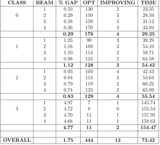
4.1 Branch-and-price results for Classes 0, 1, and 2 . . . 50

4.2 Branch-and-price results for Class 3 . . . 50

4.3 Beam search results . . . 52

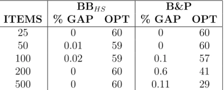
4.4 VCSBPPresults: comparison between BBHS and branch-and-price . 53

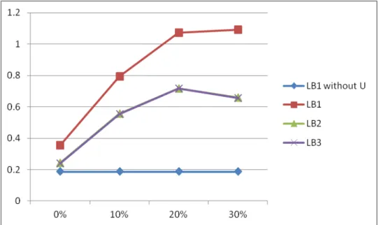
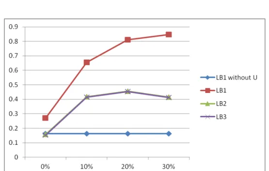
3.1 Class 4 gaps betweenZSC andLB1,LB2, andLB3 for varyingU with

a time limit of 20 seconds . . . 36

3.2 Class 4 gaps betweenZSC andLB1,LB2, andLB3 for varyingU with

a time limit of 1000 seconds . . . 37

Introduction

Packing problems make up a fundamental topic of combinatorial optimization. Their importance is confirmed both by their wide range of scientific and technological ap-plications they are able to address and by their theoretical imap-plications. In fact, they are exploited in many fields such as computer science and technologies [Ullman,

1971, Francis, 1993, Hutton, 1993], industrial applications [Boutevin et al., 2003,

Freire Beirão, 2009], transportation and logistics [Akkas, 2004, Cochran and Ra-manujam,2006,Epstein,2009,Baldi et al.,2012c], and telecommunications [Huang and Zhuang, 2000, Skorin-Kapov, 2007, Detti et al., 2009]. From a theoretical per-spective, packing problems often appear as sub-problems in order to iteratively solve bigger problems [Naddef and Rinaldi,2001, Fukunaga and Korf, 2007].

Roughly speaking, they consist in loading a set of items into proper bins in order to optimize a given objective function. Fundamentally, packing problems can be classified into two families: the one of bin packing problems and the one of knapsack problems. These two families are very different in terms of formulations, objective functions, methodologies, and, above all, items nature. In fact, whilst in bin packing problems items are compulsory (i.e., they all must be loaded into bins), in knapsack problems they are non-compulsory.

Although packing problems play a fundamental role in all the aforementioned settings, there is a gap in terms of comprehensive study in the literature. In fact, the joint presence of both compulsory and non-compulsory items has not been con-sidered yet. This particular setting arises in many real-life applications, not yet

addressed or only partially addressed by the current state-of-the-art packing prob-lems. Furthermore, little has been done in terms of unified methodologies, and different techniques have been used in order to solve packing problems with differ-ent objective functions. In particular, none of these techniques is able to address the presence of compulsory and non-compulsory items at the same time.

In order to overcome a noteworthy portion of this gap, we formulated a new packing problem, named theGeneralized Bin Packing Problem(GBPP),

char-acterized by both compulsory and non-compulsory items, and multiple item and bin attributes.

Packing problems have also been studied within stochastic settings where the items are affected by uncertainty. In these settings, there are fundamentally two kinds of stochasticity concerning the items: 1) stochasticity of the item attributes, where one attribute is affected by uncertainty and modeled as a random variable or 2) stochasticity of the item availability, i.e., the items are not known a priori but they arrive on-line in an unpredictable way to a decision maker.

Although packing problems have been studied according to these stochastic vari-ants, the GBPPwith uncertainty on the items is still an open problem. Moreover,

to the best of our knowledge, also the on-line variant of the VCSBPP, the most

similar problem to the GBPP, has not been studied yet. Therefore, we have also

studied two stochastic variants of theGBPP, named theStochastic Generalized Bin Packing Problem (S-GBPP) and the On-line Generalized Bin Packing Problem (OGBPP), and the on-line variant of the Variable Cost and Size Bin Packing Problem (VCSBPP), theOn-line Variable Cost and Size Bin Packing Problem (OVCSBPP).

Our main results concern the development of models and unified methodolo-gies of these new packing problems, making up, as done for the Vehicle Rout-ing Problem (VRP) with the definition of the so called Rich Vehicle Routing Problems, a new family of advanced packing problems named Generalized Bin Packing Problems.

In the GBPP, a set of items, characterized by volume and profit, and a set of

bins, characterized by capacity and cost, are given. The item set is split into two subsets: the subset of compulsory items (which must be loaded into bins) and the subset of non-compulsory items (which may not be loaded). The bins are classified

by types, such that bins belonging to the same type have the same capacity and cost. The goal is to properly select a subset of profitable non-compulsory items to be loaded together with the compulsory ones into the appropriate bins in order to minimize the total net cost and satisfying capacity and bin usage constraints. The total net cost is given by the difference between the total cost of the selected bins and the total profit of the loaded non-compulsory items.

The GBPP yields a relevant amount of contributions. The most relevant

con-tribution is the presence of both compulsory and non-compulsory items and of mul-tiple item and bin attributes. This innovative feature allows us to address and collect several bin packing and knapsack problems at the same time into a unique structure. The GBPP, indeed, is able to gather the following packing problems:

the Bin Packing Problem(BPP), theVariable Sized Bin Packing Problem

(VSBPP), the VCSBPP, the Knapsack Problem (KP), theMultiple Knap-sack Problem (MKP), and the Multiple Knapsack Problem with identical capacities (MKPI). Moreover, the GBPP is able to address new applications.

In logistics, where changes arising in the supply chain and fleet management due to cross-continental fleet flows and multi-modal and green logistics have forced re-searchers and practitioners to redefine their processes [Cohn and Barnhart, 1998,

Shintani et al., 2007]. TheGBPPis a contribution in this direction, as it defines a

packing problem able to simultaneously consider bin costs and item profits and takes into account restrictions on the bin availability and their heterogeneity in terms of cost and volume. The GBPP brings also innovation in the area of airfreight

trans-portation, where items are loaded according to their volume [Li, 2011]. Here, the

GBPP is able to describe the fundamental role played by the trade-off between

shipping costs and item profits, which arises in many transportation settings. The

GBPP also brings contributions in the waste collection problem at a tactical level.

In the literature, this problem is tackled at the operational level, where the routes are determined solving a VRP [Bianchi de Aguiar, 2010, Bianchi de Aguiar et al., 2012]. Given the demand of ordinary waste and hazardous and bulky waste (which yield a profit to the waste company), the GBPP determines proper vehicles

(rep-resented by bins) in order to fulfill an optimized picking. Afterward, routes are determined at the operational level, solving the VRP.

terms of quality and computational time.

Furthermore, the availability of these methodologies for the GBPP yields the

great flexibility of using the same techniques to address different problems, avoiding to change the solution methods every time the problem changes.

The Stochastic Generalized Bin Packing Problem is a further

generaliza-tion of theGBPPwhere item profits are no longer fixed, but depend on bins where

items will be loaded. Moreover, they are random variables with unknown probabil-ity distribution. The goal is to maximize the expected total net profit, given by the difference between the expected total profit of the loaded items and the total cost of the used bins, while satisfying volume and bin availability constraints.

The S-GBPP is able to address a more general setting where each item profit

depends on the bin where the item is loaded and it is described by a random variable. This generalization allows us to address new applications, in particular in logistics, where the freight consolidation is essential to optimize the delivery process. Profit random terms represent a series of handling operations for bin loading that must be performed at the logistic platforms, and these operations could significantly affect the final total profit of the loading [Tadei et al., 2002].

Moreover, the S-GBPPis able to address the Railway Track Maintenance Planning Problem, where maintenance operations (named warnings) must be

scheduled into time-slots and their costs are uncertain and depend on the time-slots where they are assigned [Heinicke et al., 2012, 2013].

For this problem, we give a stochastic model and, applying the extreme value theory, we derive a deterministic approximation.

In the On-line Generalized Bin Packing Problem, the items arrive on-line

to a decision maker, therefore no information on the items is known a priori. Only when an item has been received, its information is revealed.

This problem arises in all those applications where orders arrive on-line. This is the case, for instance, of freight forwarders: specialized companies arranging ship-ments between logistics providers and customers, and playing the role of intermedi-ary between the involved parts.

We study a wide range of algorithms in order to test whether the available tools in the literature (i.e., the asymptotic and absolute worst case ratios) are still effec-tive when a richer setting as the OGBPP is tackled. Our study reveals a stronger

result than the one achieved in the On-line Knapsack Problem(OKP). In fact,

as Iwama and Zhang [2007, 2010] showed that the OKP is not competitive (i.e.,

its absolute worst case ratio is infinite), we prove that, for the proposed algorithms, it is even impossible to apply the definition of these tools. This behavior occurs also in the On-line Generalized Bin Packing Problem with item profits proportional to item volumes (OGBPPκ), the on-line variant of the

General-ized Bin Packing Problem with item profits proportional to item volumes

(GBPPκ), a particular case of the GBPP where item profits are proportional to

their corresponding volumes through a positive coefficient κ. This particular prob-lem arises in many real-life applications.

We believe that the ultimate packing problem for which it is possible to com-pute a performance ratio is the On-line Variable Cost and Size Bin Packing Problem, the closest problem to the GBPP, where items arrive on-line, but still

without the presence of non-compulsory ones. As for the OGBPP, this problem

arises in many settings where orders arrive on-line.

For this problem, we could generalize the work of Li and Chen[2006] to a more general setting, still guaranteeing the same performance ratio.

This thesis is organized as follows. In Chapter 2, we present a detailed state of the art of the GBPP and of the packing problems it is able to address.

In Chapter 3, we present the GBPP. After introducing the problem, we give

two models and propose bounds. In particular, we propose two lower bounds, one solving anAggregate Knapsack Problem(AKP) and a second one computed in

terms of column generation. Then, we show how, basing on these lower bounds, we can also compute accurate upper bounds. We also compute upper bounds in terms of constructive heuristics. Afterwards, we present new instance sets for tackling the problem and extensive computational results.

In Chapter 4, we give an exact method, named branch-and-price, for solving the GBPP. Our method, rooted on a previous work of Bettinelli et al. [2010],

consists in a two-layer branching strategy. We also propose an approximate method, named beam search, which is based on the branch-and-price architecture. Extensive computational results are also presented.

In Chapter 5, we present the S-GBPP. We first provide a more general

where it is loaded. Then, we present the stochastic model, where each profit be-comes a random variable with unknown distribution. Starting from this model and applying the extreme value theory, we derive a deterministic approximation of the

S-GBPP.

In Chapter 6, we present the OGBPP, the OGBPPκ, and the OVCSBPP,

and we propose and study a wide range of algorithms addressing these problems. Conclusions and future developments of the research activity are reported in Chapter 7.

Literature review

In this chapter, we recall the literature of the GBPP and of its related problems.

These are: the BPP, the VSBPP, the VCSBPP, the KP, the MKP, and the

MKPI.

TheGBPPis a novel packing problem recently introduced byBaldi et al.[2012a].

In their paper, the authors propose two models and preliminary bounds. A branch-and-price method and beam search heuristics have been proposed in [Baldi et al.,

2012b]. The stochastic variant of the problem has been studied by Perboli et al.

[2012].

The most classical bin packing problem addressed by theGBPPis theBPP. The BPP is the simplest mono-dimensional bin packing problem, introduced byUllman

[1971], which consists in finding the minimum number of bins (all having the same capacity) in order to accommodate a set of items satisfying capacity constraints. A noteworthy pioneering work has been conducted by Johnson who, in his papers and PhD thesis, proposed and studied preliminary algorithms, some of them still in the vanguard. In particular, in [Johnson, 1973a], he proposed the Next Fit (NF)

algorithm and proved that its performance ratio is 2. In [Johnson et al., 1974], he proposed the First Fit (FF), Best Fit (BF), First Fit Decreasing(FFD),

and Best Fit Decreasing(BFD) algorithms and showed that their performance

ratios are, 17/10 for FF and BF and 11/9 for FFD and BFD. FFD and BFD

are still very used nowadays, sometimes combined with local improvement heuris-tics [Schwerin and Wäscher, 1997]. Basing their studies on the work of Johnson,

several authors proposed improved algorithms in the years. Yao [1980] presented the Refined First Fit algorithm, with performance ratio 5/3, and proved that

any on-line algorithm must have a performance ratio of at least 3/2. Afterward,van Vliet [1992] increased the lower bound to 1.54014. Lee and Lee [1985] presented a family of bounded space algorithms, named HarmonicM, with performance ratio

approaching h∞ ≈ 1.6910 from above as M → +∞, and showed that h∞ is even a lower bound for this class of problems. The authors also presented the Refined Harmonic algorithm, with performance ratio 373/228 ≈ 1.63597. To the best of

our knowledge the best result to date is due to Seiden [2002] who proposed the

Harmonic++ algorithm with performance ratio at most 1.58889.

Preliminary bounds to the BPP were proposed by Martello and Toth [1990].

New lower bounds were developed by Fekete and Schepers [2001] by means of dual feasible functions. On the basis of this paper, Crainic et al. [2007] developed fast and more accurate lower bounds, able to reduce the optimality gap for a number of hard instances. A different approach was defined in [Vanderbeck, 1996], where the author proposed a formulation with an exponential number of variables and a column generation lower bound procedure for the Bin Packing and the Cutting Stock problems. Several heuristics were also proposed [Martello and Toth, 1990], e.g., the polynomial-time approximation schemes of de la Vega and Lueker [1981] andKarmarkar and Karp[1982] allowing to approximate an optimal solution within 1 +, for any fixed >0. However, these results are difficult to apply in practice, due to the enormous size of the constants characterizing the polynomials.

Han et al.[2010] studied a variant of the problem where items have also arrival and departure time. Both the off-line and the on-line versions of the problem were studied, with particular attention to the case of unit fraction items, i.e., when the sizes of the items are at most 1/i, for some integer i.

TheBPPhas also been studied with respect to less standard ratios. Epstein and van Stee [2005] studied the problem by means of resource augmentation. Kouakou et al. [2005] studied the problem with respect to the differential competitivity ratio. Finally, György et al. [2010] studied a much more restrictive variant of the problem with just one open bin and the decision maker can only decide whether to pack the next item into the open bin or close the incumbent open bin and load the item into a new bin (which, of course, becomes the new open bin). If the decision maker decides

not to close the current open bin and the next item does not fit into it, then the item is lost. The goal is to minimize the wasted space plus the number of lost items. This version of the problem is called on-line Sequential Bin Packing Problem.

Another variant of the BPP was studied by Li and Chen [2006], where the

bins have all the same capacity but they are also characterized by a non-decreasing concave cost function. The authors proved that, for this variant of the problem,

FF and BF heuristics have absolute worst case ratio equal to 2, whilst FFD and BFD have absolute worst case ratio equal to 1.5. For this problem, Leung and Li [2008] developed a polynomial time approximation algorithm such that, for any positive , the asymptotic worst case ratio is 1 +. Epstein and Levin [2012] have recently designed an asymptotic fully polynomial time approximation scheme for this problem. In their work, the authors have also proposed a fast approximation algorithm with asymptotic worst case ratio of 1.5.

The stochastic variant of the BPP has been studied by Coffman Jr. et al.

[1980], Lueker [1983],Rhee and Talagrand [1993a,b]. In these papers, the source of uncertainty is the item volume and strong hypotheses on the probability distribution of the random terms are usually done. Recently,Peng and Zhang[2012] have studied a more general stochastic variant, where both item volumes and bin capacities are uncertain.

Another problem addressed by the GBPP is the VSBPP, where bins with

different sizes are available and the goal is to minimize the wasted space. This problem was first investigated byFriesen and Langston[1986]. The authors provided one on-line and two off-line algorithms and proved that their worst case ratio is respectively 2, 3/2, and 4/3. Murgolo [1987] presented an approximation scheme which, for any positive, produces a scheme with performance ratio 1+. Moreover, his algorithm is polynomial even with respect to 1/. Chu and La [2001] proposed four greedy approximation algorithms with absolute worst case ratio respectively equal to 2, 2, 3, and 2 + ln 2. The authors also showed that these bounds are tight.

Seiden[2000] proposed an optimal on-line algorithm for the bounded space (i.e., the number of open bins is constant) problem. Seiden et al. [2003] proposed improved bounds but with two bin sizes only. Zha provided a lower bound of 2.245 with respect to the absolute worst case ratio and proposed a simple on-line algorithm with absolute worst case ratio equal to 3. The author also studied the problem from

another point of view: if one were allowed to design k bin sizes, what sizes should be chosen such that, for any instance, the wasted space is minimized?

Monaci [2002] presented a series of lower bounds and solution methods (both heuristic and exact) for the VSBPP. The author also introduced instance sets for

the problem considering up to 500 items. His exact method was able to solve most instances to optimality.

The VSBPP can also be seen as a special case of the Multiple Length Cutting

Stock Problem(MLCSP). In this problem, the item demand can be more than one and different types of stocks (which are equivalent to the bins) are available. Exact methods for the MLCSP have been proposed byBelov and Scheithauer[2002]. Alves and Valério de Carvalho [2007] first proposed an improved column generation tech-nique trying to solve the VSBPP to optimality. One year later, the same authors

introduced a branch-and-cut-and-price algorithm for the MLCSP [Alves and Valério de Carvalho,2008].

An on-line variant of theVSBPP was introduced by Zhang[1997] where items

are known and this time are the bins to arrive on-line, one by one. The author proved that, for this problem, both NF and FFD algorithms have performance

ratio 2.

The problem studied by Zhang [1997] was also the starting point for the work of Epstein et al.[2011] who studied the on-line Variable Sized Bin Packing Problem with conflicts.

The VCSBPP is a generalization of the VSBPP, where all items must be

loaded, but bins can be chosen among several types differing in volume and cost. The total accommodation cost, computed as the total cost of the used bins, must be minimized. A number of studies have been dedicated to the VCSBPP. Kang and Park [2003] studied the problem assuming that the cost of the unit size of each bin does not increase as the bin size increases. The authors proposed two greedy algorithms and computed their asymptotic worst case ratio under three assumptions: 1) the sizes of items and bins are divisible (i.e., the succeeding item (bin) exactly divides the previous item (bin)), 2) the sizes of bins are divisible, and 3) the sizes of bins are not divisible. The authors proved that both algorithms yield an asymptotic worst case ratio equal to 1 (i.e., the two algorithms are optimal) under assumption 1, equal to 11/9 under assumption 2, and equal to 3/2 under assumption 3. For

this problem, Epstein and Levin [2008] designed an asymptotic polynomial time approximation scheme. Correia et al. [2008] proposed a formulation that explicitly includes the bin volumes occupied by the corresponding packings, together with a series of valid inequalities improving the quality of the lower bounds obtained from the linear relaxation of the proposed model. The authors also introduced a large set of instances with up to 1000 items and used them to analyze the quality of the lower bounds. Crainic et al. [2011] proposed tight lower and upper bounds, which can be computed within a very limited computing time, and were able to solve to optimality all the instances proposed in [Correia et al.,2008]. The authors also presented a first computational study of the sensitivity of the optimal cost with respect to the cost definition [Crainic et al., 2011]. Approximation algorithms have been proposed by

Haouari and Serairi[2009] andHemmelmayr et al.[2012]. Recently, Bettinelli et al.

[2010] introduced a branch-and-price algorithm for the resolution of a variant of the

VCSBPPwith the addition of filling constraints. These constraints imply that, due

to stability reasons within the bins, each bin must be filled at least at a minimum security level. To the best of our knowledge, the latest work dealing with exact methods for solving the VCSBPP is due to Haouari and Serairi [2011], in which

the authors proposed lower bounds and an exact branch-and-bound algorithm. Fazi et al. [2012] have recently studied the Stochastic VCSBPP, with the addition of

time constraints.

The GBPP is also able to generalize three knapsack problems: the KP, the MKP, and the MKPI. The KP is a deeply studied Combinatorial Optimization

problem where, given a set of items characterized by volume and profit, the goal is to find a proper subset such that the profit is maximized and the sum of volumes of the selected items does not exceed the capacity of the only available bin, namely the knapsack. TheMKP is a generalization of the KP due to the presence of more

than one knapsack. Finally, the MKPI is a particular case of the MKP, where all

the knapsacks have the same capacity. All these problems are thoroughly discussed in [Martello and Toth, 1990, Pisinger,1995, Kellerer et al., 2004].

The OKP has been studied by Iwama and Taketomi [2002], Iwama and Zhang

[2007,2010]. In these papers, the authors prove that, for this problem, the worst case ratio is infinite. For this reason, they also study the on-line variant with removable items and resource augmentation and, for this variant of the problem, the proposed

algorithms show finite competitive ratios.

In the stochastic variant of the problem, named the Stochastic Knapsack Problem (SKP), the source of uncertainty is usually the item profit, and strong hypotheses on

its probability distribution are made [Goel and Indyk,1999,Ross and Tsang,1989]. Some papers also consider the item volume stochasticity. Dean et al.[2008] present some policies to decide whether to load the items into the knapsack, showing how an adaptive loading policy outperforms a non-adaptive one. In Kosuch and Lisser

[forthcoming], a variant of the SKPwith normally distributed volumes is presented.

The authors derive a two-stageSKPwhere, contrary to the single-stageSKP, items

can be added to or removed from the knapsack at the moment the actual volumes become known (second stage).

The Generalized Bin Packing

Problem: models and bounds

In this chapter, we introduce the GBPP together with models and bounds. After

defining the problem in a formal way, we present two mixed integer programming formulations. The first is based on item-to-bin assignment decisions and requires a polynomial number of variables and constraints. This formulation shows how the

GBPP generalizes several packing problems, but is not computationally efficient.

It is, however, the starting point for computing the first lower bound. Moreover, it is also the starting point for the S-GBPP, introduced in Chapter 5. We, thus, introduce a second model, based on feasible loading patterns and set covering ideas. Despite requiring an exponential number of variables, this formulation is much more efficient. We then present several procedures in order to compute lower and upper bounds to the GBPP and show their accuracy and efficiency through extensive

computational experiments. A large number of instance sets for the GBPP are

introduced. The instance sets are designed to challenge the proposed procedures and thus provide insight into the impact of different parameters on the optima.

This chapter is organized as follows. The two GBPP formulations are

intro-duced in Section 3.1; lower and upper bounds are presented in Sections3.2 and 3.3, respectively. Instance sets and computational results are presented and discussed in Section 3.4.

3.1

Problem Definition and Formulation

The GBPP considers a set of items characterized by volume and profit and sets of

bins of various types characterized by volume and cost. A subset of the items which we call compulsory must be loaded, while a selection has to be made among the non-compulsory ones. The objective is to select the non-compulsory items to load

and the bins into which to load the compulsory and the selected non-compulsory items in order to minimize the total net cost. This is given by the difference between the total cost of the used bins and the total profit of the loaded items.

In this section, we present a formal description of the GBPP and we introduce

two formulations of the problem. The first formulation extends to the GBPP the

assignment model of the BPP [Martello and Toth, 1990]. Although this kind of

formulation is not often used in practice, we exploit it to derive a first lower bound. Then, we consider a set covering formulation of the problem, which is the starting point for a column generation procedure, which allows us to derive a second lower bound and upper bounds as well.

3.1.1

Notation

Let I denote the set of items and wi and pi be the volume and profit of item i∈ I.

Define IC _{⊆ I the subset of compulsory items and I}NC _{= I \ I}C _{the subset of}

non-compulsory items. Let J denote the set of available bins and T be the set of

bin types. For any bin j ∈ J, let σ(j) = t ∈ T be the type t of bin j. Define, for each bin type t ∈ T, the minimum Lt and the maximum Ut number of bins of

that type that may be selected, as well as the cost Ct and the volumeWt of the bin.

Finally, denote U ≤P

t∈T Ut the total number of available bins of any type.

The item-to-bin accommodation rules of theGBPP are stated as follows

• All items inIC _{must be loaded}

• For all used bins, the sum of the volumes of the items loaded into a bin must be less than or equal to the bin volume

• The number of bins used for each type t ∈ T must be within the lower and

• The total number of used bins cannot exceed the total number of available bins U.

Infeasibility may arise when the available bins are not sufficient to load all com-pulsory items. To address this issue, we add a special bin v of volume Wv =

P

i∈ ICw_i, thus able to load all compulsory items, and set its cost C_v to a value much higher than the costs of the remaining bins in order to discourage its use, e.g., Cv Pt∈ T Ct.

3.1.2

Assignment formulation of the GBPP

• Bin selection binary variablesyj equal to 1 if bin j ∈ J is used, 0 otherwise

• Item-to-bin assignment binary variables xij equal to 1 if item i ∈ I is loaded

into bin j ∈ J, 0 otherwise.

An assignment model of theGBPP can then be formulated as follows

min X j∈J Cjyj − X j∈J X i∈INC pixij (3.1) subject to X i∈I wixij ≤Wjyj j ∈ J (3.2) X j∈J xij = 1 i∈ IC (3.3) X j∈J xij ≤1 i∈ INC (3.4) X j∈J:σ(j)=t yj ≤Ut t∈ T (3.5) X j∈J:σ(j)=t yj ≥Lt t∈ T (3.6) X j∈J yj ≤U (3.7) yj ∈ {0,1} j ∈ J (3.8) xij ∈ {0,1} i∈ I, j ∈ J. (3.9)

The objective function (3.1) minimizes the total net cost of the packing, given by the difference between the total cost of the used bins and the total profit of the selected non-compulsory items. The profit of the compulsory items is not considered in the objective function because it is a constant. Regarding the type of optimization, we choose to present the minimization version to follow the tradition of bin packing problems. The equivalent formulation obtained by maximizing the total net profit (total profit minus total cost) would recall the knapsack problem setting.

Constraints (3.2) have the double effect of linking the usage of bins to the ac-commodation of items and bounding the capacity of each used bin. Constraints (3.3) and (3.4) ensure that each compulsory and not-compulsory item is loaded into exactly one and at most one bin, respectively. Constraints (3.5) and (3.6) enforce the maximum and minimum number of available bins of each type, while Constraint (3.7) limits the total number of selected bins. Constraints (3.8) and (3.9) enforce the integrality nature of the decision variables. Notice that, Constraints (3.5) and (3.6) could be implicitly managed, the former by limiting the number of yj

vari-ables to Ut for type t (i.e., defining the appropriate number of bins only), and the

latter by setting yj = 1 for j = 1, . . . , Lt. We prefer to keep the constraints in the

formulation, however, for consistency with the set covering model of Section 3.1.4. The assignment model (3.1)-(3.9) is named AM and its continuous relaxation R-AM. AM involves a polynomial number of variables and constraints. It is not

suitable for developing efficient algorithms, however, due to the significant solution-space symmetry of the item-to-bin assignment variables, which is typical of these packing models. Yet, as mentioned above, AM is the starting point to compute

our first lower bound named LB1 and to formulate the S-GBPP in Chapter 5.

Furthermore, AM is also suitable to show how the _GBPP generalizes some classic

bin packing and knapsack problems. This issue is addressed next.

3.1.3

Generalization of classic bin packing and knapsack

problems

The assignment formulation (3.1)-(3.9) is useful to show how the GBPP can

gen-eralize a number of classic packing problems. As mentioned in Chapters 1 and 2, the GBPP is able to address theBPP, the VSBPP, the VCSBPP, the KP, the

MKP, and the MKPI. The BPP can be modeled by considering a single bin type

with Cj = 1, j ∈ J and INC =∅, i.e., all items must be loaded. Constraints (3.4)

- (3.6) are then redundant and the objective function becomes the minimization of the number of bins, which is characteristic of the BPP.

Allowing several bin types andINC =_∅yields the

VCSBPP, where the total cost

of the selected bins P

j∈J Cjyj is minimized (Constraints (3.4) become redundant)

[Monaci, 2002, Crainic et al., 2011]. Notice that, an equivalent formulation for the

VCSBPP can be obtained by imposing IC = ∅ and setting the item profit higher

than the cost of any bin type, pi >maxj∈J Cj, which makes any bin profitable even

when only one item is loaded into it.

The VSBPP can also be addressed setting INC=∅ and Cj =Wj, ∀j ∈ J.

TheGBPPcan similarly generalize a number of knapsack problems. Specifically,

the GBPPreduces to the KP by setting |T | = 1,|J | = 1, and IC =∅. The MKP

can be modeled by setting |T |>1, |J |=m, where m is the number of knapsacks, and IC = _∅. Finally, the MKPI is addressed by setting _{|T |} = 1, _{|J |} = _m, and IC =_∅.

3.1.4

Set Covering formulation of the GBPP

We introduce a set covering formulation of the GBPP based on feasible loading

patterns for the bins.

Afeasible loading pattern kt for a bin of typet ∈ T is a set of items that may be

loaded into the bin while satisfying all dimension restrictions and accommodation rules. Let Kt = {kt} be the set of all feasible loading patterns for bin type t ∈ T.

A feasible loading pattern kt is described by a vector akt of indicator functions ai

kt, i ∈ I, kt ∈ Kt, t ∈ T, such that a

i

kt = 1 if item i is packed into pattern kt, 0

otherwise. The cost of pattern kt is then the difference between the cost of the bin

type t and the total profit of non-compulsory items in that pattern: ckt =Ct−

X

i∈INC

piaikt. (3.10)

We define the bin loading pattern selection variables λkt equal to 1 if pattern

be written as follows min X t∈T X k∈Kt cktλkt (3.11) subject to X t∈T X k∈Kt ai_ktλkt = 1 i∈ I C _{(dual variable µ} i free) (3.12) X t∈T X k∈Kt ai_ktλkt ≤1 i∈ I NC_{(dual variable ν} i ≤0) (3.13) X k∈Kt λkt ≤Ut t ∈ T (dual variable αt≤0) (3.14) X k∈Kt λkt ≥Lt t ∈ T (dual variable βt≥0) (3.15) X t∈T X k∈Kt λkt ≤U (dual variable≤0) (3.16) λkt ∈ {0,1} kt ∈ Kt, t∈ T. (3.17)

The objective function (3.11) minimizes the total cost of the selected bin loading patterns.

Since the feasibility of the item-to-bin accommodation is guaranteed by the fea-sibility of the loading patterns, the constraints equivalent to (3.2) in the model

AM are not required anymore. Constraints (3.12)-(3.16) have the same meaning as

(3.3)-(3.7), and (3.17) are the integrality constraints.

The set covering model (3.11)-(3.17) is namedSC and its continuous relaxation R-SC. SC, when compared to AM, has the advantage to separate the feasibility

phase from the optimality one. The feasibility phase is already addressed by the pattern generation, whilst the model is only devoted to find an optimal combination of patterns.

Whilst, of course, models AM and SC have the same optimum, the optima of R-AM and R-SC are generally different. In the following, we prove that the lower

bound to theGBPPobtained by optimizingR-SC is not weaker than that obtained

by optimizing R-AM.

Property 1. Given any solution x2 of R-SC (which is feasible by construction),

a corresponding feasible solution x1(x2) of R-AM can be built as follows. For any

ai_ktλkt in the solution x1(x2). The two solutions have the same value.

Proof. Trivial.

Theorem 1. Let LR-AM = optimum(R-AM) and LR-SC = optimum(R-SC), then

LR-AM ≤LR-SC.

Proof. By contradiction, let us suppose that an instance ofR-AM such thatLR-AM > LR-SC there exists. Let x2 be the optimal solution associated to LR-SC. By using Property 1, we can build a solution x1(x2) of R-AM with value LR-SC, which con-tradicts the optimality of LR-AM.

3.2

Lower bounds

We introduce two lower bounds that can be computed starting from each of the two problem formulations. The assignment model AM is the basis for a lower bound

which can be calculated by solving an Aggregate Knapsack Problem (AKP). We show how to derive the AKP from the model AM in Section 3.2.1.

The second lower bound is derived from the set covering formulation SC and is

calculated by applying a column generation technique where, at each step, a new feasible pattern (i.e., a new column for the restricted master problem) is found by solving a knapsack problem (see Section 3.2.2).

3.2.1

Lower bound through the Aggregate Knapsack

Prob-lem

To derive an Aggregate Knapsack Problem from the assignment model AM

pre-sented in Section 3.1.2, we aggregate Constraints (3.2) into a unique inequality by summing them up. We thus consider an aggregate knapsack, which may be thought of as a unique large bin with volume equal to the total volume of the bins. We have

X j∈ J X i∈ I wixij ≤ X j∈ J Wjyj =⇒ X i∈ IC wi X j∈ J xij+ X i∈ IN C wi X j∈ J xij ≤ X j∈ J Wjyj.

Note that, by (3.3), for any compulsory item i, X

j∈ J

xij = 1, whilst, for any

non-compulsory item i, the variable xij can be reduced toxi, which states whether item

i is put into the aggregate knapsack or not. Therefore, we have

X i∈ IC wi+ X i∈ IN C wixi ≤ X j∈ J Wjyj. (3.18)

We drop Constraints (3.5) and (3.6) by implicitly managing them as indicated in Section3.1.2. Constraint (3.7) is kept, as one cannot implicitly manage it. A first lower bound, named LB1, can then be found by solving the following AKP

min X j∈J Cjyj − X i∈INC pixi (3.19) subject to X i∈ IC wi+ X i∈ IN C wixi ≤ X j∈ J Wjyj (3.20) X j∈J yj ≤U (3.21) yj ∈ {0,1} j ∈ J (3.22) xi ∈ {0,1} i∈ INC. (3.23)

Since LB1 comes from the resolution of the AKP, we also refer to it as an

aggregate knapsack lower bound. Note that, when all items are compulsory, one can

use bounds from the literature. In this case, (3.19)-(3.23) reduces to

min X j∈J Cjyj (3.24) subject to X i∈ IC wi ≤ X j∈ J Wjyj (3.25) X j∈J yj ≤U (3.26) yj ∈ {0,1} j ∈ J, (3.27)

which is the model used by Crainic et al. [2011] to compute lower bounds to the

3.2.2

Lower bound through column generation

This lower bound is computed from the R-SC model through column generation

and is named LB2. It is widely used in bin packing problems [Alves and Valério de Carvalho, 2007, Vanderbeck, 1996] and provides the means to implicitly deal with a large number of variables.

The column generation approach applied to theR-SC model consists in starting

with a relatively small set of feasible patterns P, which correspond to a restricted

problem named R−SCR. First we solve R−SCR and then attempt to generate

new feasible patterns with negative reduced cost. If successful, these are added to

P and the procedure is restarted. Otherwise, we have found an optimal solution of

R-SC and the procedure stops with a lower bound to the _GBPP.

The main steps of the procedure are as follows

1. Find an initial feasible solution of the GBPPand the corresponding set P

2. Solve to optimalityR−SCR and let LR−SCR be its optimum

3. For each bin type t∈ T

(a) Find the pattern variable λ_k

t, kt ∈ Kt with the smallest reduced cost

r_k

t, among all non-basic pattern variables λkt of the optimal solution of

R−SCR

(b) Ifr_k

t <0,P =P ∪ {λkt}

4. If r_k

t ≥0 for all bin typest, then stop and LR−SCR is the lower bound to the

GBPP, otherwise, go to 2.

Note that, in Step 3, the procedure adds at most |T | columns to P at each

iteration.

The main issue is how to find negative reduced cost feasible patterns. Consider the dual variables associated to the constraints of the R−SCR model (see (3.11

)-(3.17)). The reduced cost rkt of a given pattern variableλkt is ckt −

h µT _νTi_a kt − h αT βT i1t, whereakt = [a i

kt] and 1tis a vector of size 2|T | +1, with 1 in the rows

corresponding to bin type t and in the last row, 0 otherwise. By (3.10), we expand this expression as follows

rkt = Ct− X i∈INC piaikt − h µT νTiakt − h αT βT i1t = Ct− X i∈INC piaikt − X i∈IC µiaikt − X i∈INC νiaikt−αt−βt− = Ct− X i∈INC (pi+νi)aikt − X i∈IC µiaikt −αt−βt−. (3.28)

We now define a column generation sub-problem. Given a bin of type t ∈ T,

this sub-problem finds the non-basic pattern with the minimum reduced cost. Note that, the vector akt defining a not-yet-generated pattern kt∈ Kt is not known, but it may be expressed in terms of the item-to-bin assignment variable xi, which is

equal to 1 if item i∈ I belongs to the pattern, 0 otherwise. Since the dual variables

αt, βt, and , as well as the bin cost Ct, are constant for any given bin type t ∈ T,

then finding the feasible pattern with the minimum reduced cost for bin type t∈ T

becomes the following knapsack problem max    X i∈INC (pi +νi)xi+ X i∈IC µixi    (3.29) subject to X i∈I wixi ≤Wt t∈ T (3.30) xi ∈ {0, 1} i∈ I. (3.31)

Any feasible solution may be used to initialize the procedure, including the triv-ial solution obtained by loading each compulsory item into a different bin. More accurate heuristics are presented in Section 3.3.

Finally, note that a better lower bound can be obtained by taking the maximum between the two previous lower bounds. We call this new lower bound LB3 =

max{LB1, LB2}.

3.3

Upper bounds

We derive several upper bounds to the GBPP: 1) through constructive heuristics,

generation-based heuristics.

3.3.1

Upper bounds through constructive heuristics

We propose constructive heuristics to load items into bins based either on the FFD

or the BFD heuristics for the BPP, with different sorting rules for items and bins.

We briefly recall how FFD and BFD work. Starting with items sorted by

non-increasing volume, FFD loads items one after the other into the first bin where

they fit. BFD attempts to load each item into the “best" bin, usually the bin

with the minimum free volume after loading the item. The free volume is defined

as the bin volume minus the total volume of the loaded items. Both heuristics create a new bin when an item cannot be accommodated into the existing ones. Despite their simplicity, the FFD and BFD heuristics offer good performances for

the BPP[Johnson et al.,1974, Martello and Toth,1990].

Note that, whilst in the BPP items are sorted by non-increasing volume, many

item and bin sorting rules are possible for theGBPP, due to the presence of multiple

attributes. We exploit this characteristic in building our heuristics.

Given the sorted lists of items and bins, SIL and SBL (see Section 3.3.1 for

deriving these lists), our heuristics are composed of three main components displayed in Algorithms 1, 2, and3. Given a list S of selected bins (initially empty), for each item belonging to SIL, Algorithm 1 (the _main procedure) looks for the first or the

best bin in S able to load such an item by using FFD or BFD, respectively. If

this bin exists, the item is loaded into it, otherwise a new bin is possibly selected. Actually, a new bin is selected when the item is compulsory otherwise we evaluate whether to select a new bin or not. This evaluation is performed by Algorithm 2

(the profitable procedure), which measures the profitability of the current item.

In particular, a new bin will be selected and the item will be loaded into it if the profit of this item plus the profits of the remaining non-compulsory items in SIL is greater than the cost of the new bin. Finally, the post-optimizationprocedure of

Algorithm3attempts to improve the final solution by evaluating possible bin swaps that replace loaded bins with available cheaper bins of sufficient capacity.

Algorithm 1 The _mainprocedure S :=∅

for all i∈ SIL do

Identify the bin b ∈ S into which item ican be loaded:

• FFD: the first bin with enough empty volume to accommodate item i

• BFD: the bin with the minimum free volume after loading item i if b exists then

Load item i into bin b

else

if i∈IC then

Identify the first bin b∈SBL\ S such that wi ≤Wb.

Load item i into binb

S :=S ∪ {b} else

Identify the binb ∈SBL\ S such that _profitable(i, b) returns _true

if b exists then

Load item i into bin b

S :=S ∪ {b} else

reject item i

post-optimization

Algorithm 2 The _profitableprocedure for new bin selection SILi : sublist ofSIL starting from the item i;

Load i intob and initialize the bin profitPb =pi; for all i0 ∈SILi do

if i0 can be loaded into b then

Load i0 into b and update the bin profit Pb =Pb+pi0; if Pb > cb, returntrue else return false.

Algorithm 3 The _{post-optimization} procedure for all j ∈ S do

for all k∈ J \ S do

Uj =Piloaded intojwi

if Wk ≥Uj and Ck< Cj then

Move all the items fromj tok

Building the sorted lists of items and bins

We define four sorting rules to embed into the constructive heuristics we propose. All the rules have in common that compulsory items are sorted at the top of the item list by non-increasing volume. The four rules are:

1. Bins: Non-decreasing Cj/Wj and non-decreasing volumesWj

Non-compulsory items: Non-increasingpi/wi and non-increasing volumes

wi

2. Bins: Non-decreasing Cj/Wj and non-decreasing volumesWj

Non-compulsory items: Non-increasing volumeswiand non-increasingpi/wi

3. Bins: Non-decreasing Cj/Wj and non-increasing volumesWj

Non-compulsory items: Non-increasingpi/wi and non-increasing volumes

wi

4. Bins: Non-decreasing Cj/Wj and non-increasing volumesWj

Non-compulsory items: Non-increasing volumeswiand non-increasingpi/wi.

3.3.2

Upper bounds through the lower bound

LB

To derive an upper bound from LB1, introduced in Section 3.2.1, we apply our

constructive heuristics to the two ordered lists of bins and items. We name this approach lower bound-based constructive heuristics. We refer to _L-FFD and L-BFD when the constructive heuristics, which is based on the lower bound LB1,

implements the FFD and theBFD principle, respectively.

The ordered lists of items and bins are obtained as follows. An optimal solution of the AKP model (3.20)-(3.23) consists in a set of non-compulsory items, Iagg,

and a set of bins, Jagg. Iagg contains the non-compulsory items associated to the

variables xi equal to 1 in the optimal solution of the AKP. Similarly, Jagg contains

the bins associated to the variablesyj equal to 1 in the optimal solution of the AKP.

We then extract two subsets I0

agg and Jagg0 by selecting δi % of items in Iagg and

δb% of bins in Jagg, respectively. We then randomly select a particular sorting rule

• Order the items in I0

agg according to s and put them at the top of the item

list, before any non-compulsory item. Then, order the remaining itemsI \ I0

agg

according to s • Order the bins in J0

agg according tos and put them at the top of the bin list.

Then, order the remaining bins J \ J0

agg according tos.

To state that L-FFD and L-BFD are characterized by δi, δb, and s, we write L-FFD

δi_{, δ}b_{, s and}

L-BFD

δi_{, δ}b_{, s. The values of δ}i _{and δ}b _{are obtained by}

calibration (see Section 3.4.3 for details), whilst s ∈ {1, 2, 3, 4}, according to the

four sorting strategies presented in Section 3.3.1.

3.3.3

Upper bounds through column generation-based

heuris-tics

We present two approaches to compute upper bounds starting from the column generation-based solution of the relaxation R-SC of the set covering model SC

(3.11)-(3.17).

The first approach is to solve SC exactly, e.g., by branch-&-bound, considering

only the columns obtained by the column-generation procedure while computing the lower bound. This may still be quite time consuming, however. Consequently, we might stop with the branch-&-bound after a given computing time and name ZSC

the resulting value of the objective function, which is an upper bound to theGBPP.

The second approach is based on diving, a well-known method for finding good

quality integer solutions from the optimal continuous solutions [Atamturk and Savels-berg, 2005]. The working principle is to iteratively round up variables and re-optimize the continuous relaxation.

The diving heuristics assumes that the optimal bin loading patterns of theGBPP

are in the restricted set corresponding to the R − SCR, and iteratively slightly

perturbs the optimal continuous solution by fixing to integer some pattern-selection variables. The key feature is how to choose the variables to be fixed. Two strategies are obtained by selecting among the non-integral pattern variables the ones which maximize the expressions (3.32) and (3.33). This generates two diving heuristics named Diving1 and Diving2, which are included in the final comparative experiments

of Section 3.4: X i∈INC νiaikt+ X i∈IC µiaikt (3.32) (1−λkt)   X i∈INC νiaikt + X i∈IC µiaikt   (3.33)

3.4

Computational results

The goal of the numerical experiments is to explore the performance of the proposed lower and upper bound procedures. Section3.4.1introduces the instance sets, whilst detailed results of different variants of the lower and upper bound procedures are given in Sections 3.4.2 and 3.4.3. We study the impact of a number of problem parameters on our best bounds in Section 3.4.4.

3.4.1

Instance classes

No instances are present in the literature for the GBPP. We generated instances,

partially based on those for the VSBPP and the BPP [Monaci, 2002, Vanderbeck, 1996, Correia et al., 2008, Crainic et al., 2011]. The instances are grouped into 5 classes:

• Class 0: 300 instances by Monaci [Monaci,2002]. We chose Monaci’s instances because they are more challenging than Correia’s [Correia et al., 2008], as shown in [Crainic et al., 2011]. Since these instances were conceived for the

VSBPP, all items of each instance are compulsory. Ten instances were

ran-domly generated for each combination of number of items, item profit, item volume, and bin type for a total of 300 instances. For the sake of completeness, we report here the details of Monaci’s instances:

– Number of items: 25, 50, 100, 200, and 500

– Item volume: I1: [1, 100]; I2:[20, 100]; I13:[50, 100]

– Item profit: not defined because all items are compulsory – Bin type:

∗ 3 types of bins, with volumes 100, 120, and 150, respectively, and costs equal to volumes

∗ 5 types of bins, with volumes 60, 80, 100, 120, and 150, respectively, and costs equal to volumes.

For each bin type t, Lt = 0 and Ut = dVtot/Vte, where Vtot is the total item

volume. No values for the total number of available bins U are given.

• Class 1: same instances of Class 0, but with all items non-compulsory and item profits generated according to the pi ∈ dU(0.5,3)wie uniform distribution.

• Class 2: same instances of Class 0, but with all items non-compulsory and item profit generated according to thepi ∈ dU(0.5,4)wieuniform distribution.

• Class 3: a selection of 12 large instances (500 items) from Class 1 and Class 2 with a representative mix of characteristics in terms of item volume, item profit, and bin types. For each instance, we randomly derived five more in-stances with 0%, 25%, 50%, 75%, and 100% of compulsory items, for a total of 60 instances.

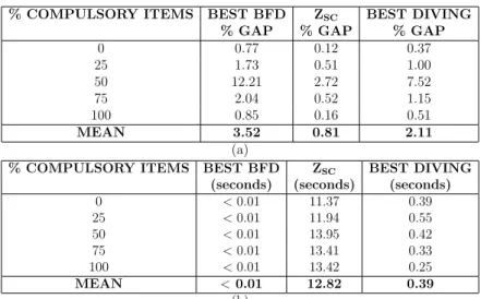
• Class 4: the aim of this class is to study the behavior of Constraints (3.7) and (3.16) on the total number of available bins U. Thus, we select 24 instances from Class 1 and Class 2. For each instance, we first computed the number of bins U employed by the _BFD constructive heuristics. We then solved the

GBPP varying the value of U as a percentage of U

U =U(1−X), X ∈ {0,0.1, 0.2, 0.3}, (3.34) All these combinations make up Class 4 with 96 instances.

The algorithms were coded in C++ and the models implemented with CPLEX 12.1ILOG Inc.[2009]. The upper boundZSC was computed using Gurobi 4.0, due to

its efficiency in finding good feasible solutions within a quite limited computing time (20 seconds) Gurobi Optimization[2010]. Experiments were made on a Pentium IV 3.0 GHz workstation with 4 GB of RAM.

3.4.2

Lower bounds

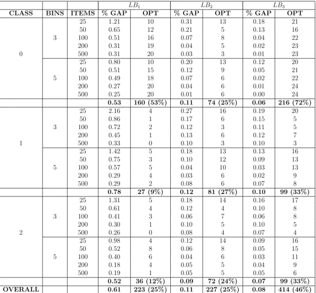
Table 3.1 shows the lower bound results, comparing the performance of the three proposed lower bounds, LB1, LB2, andLB3, relative toZSC, the best upper bound

(Section 3.3.3) or to the known optimum solution of Class 0 instances, named in the following Monaci optima [Monaci, 2002]. Columns 1 to 3 display the instance class, number of bin types, and number of items, respectively. Columns 4 and 5, 6 and 7, and 8 and 9 display the mean percentage gap to ZSC or the known optimum,

and the number of optima achieved by LB1, LB2, and LB3, respectively. Each row

of Table 3.1 gives the results of 30 instances (3 item volume types, I1, I2, and I3, times 10 repetitions). For each class and globally, the table also displays the respec-tive average gaps and the total number of optima attained (and the corresponding percentage with respect to the total number of instances).

Table 3.1 reports very promising results. The overall percentage gap for LB3 is

quite tight (0.08%) and almost half (46%) of the instances are solved to optimality.

3.4.3

Upper bounds

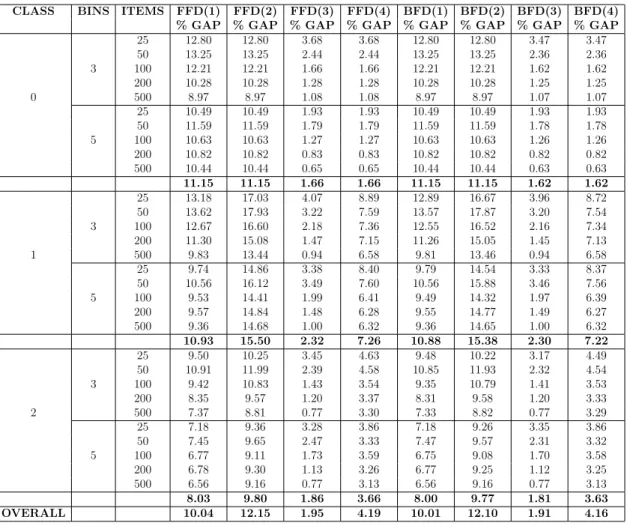
Table 3.2 displays comparative results for the constructive heuristics upper bounds. The first three columns display the same type of information as previously. Columns 4 to 7 and 8 to 11 display relative-gap results with respect toLB3(except for Class 0

instances with Monaci optima) for the FFDand the BFDprocedures, respectively,

using the four item and bin sorting rules of Section 3.3.1.

The results summed up in Table3.2show thatBFD offers slightly better results

than FFD. Furthermore, we see that BFD(3) is the best performing constructive

heuristics.

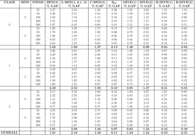
We compare the remaining upper bounds, i.e., those obtained through the lower bound LB1 (Section 3.3.2) and those derived from the column generation-based

heuristics (Section 3.3.3) in Table 3.3. Column 1 shows the instance class, Column 2 the number of bin types, and Column 3 the number of items. For the remaining columns of Table 3.3, we have:

BFD(3): BFD heuristics with the third sorting rule

LB1 LB2 LB3

CLASS BINS ITEMS % GAP OPT % GAP OPT % GAP OPT

25 1.21 10 0.31 13 0.18 21 50 0.65 12 0.21 5 0.13 16 3 100 0.51 16 0.07 8 0.04 22 200 0.31 19 0.04 5 0.02 23 0 500 0.31 20 0.03 3 0.01 23 25 0.80 10 0.20 13 0.12 20 50 0.51 15 0.12 9 0.05 21 5 100 0.49 18 0.07 6 0.02 22 200 0.27 20 0.04 6 0.01 24 500 0.25 20 0.01 6 0.00 24 0.53 160 (53%) 0.11 74 (25%) 0.06 216 (72%) 25 2.16 4 0.27 16 0.19 20 50 0.86 1 0.17 6 0.15 5 3 100 0.72 2 0.12 3 0.11 5 200 0.45 1 0.13 6 0.12 7 1 500 0.33 0 0.10 3 0.10 3 25 1.42 5 0.18 13 0.13 16 50 0.75 3 0.10 12 0.09 13 5 100 0.57 5 0.04 10 0.03 13 200 0.29 4 0.03 6 0.02 9 500 0.29 2 0.08 6 0.07 8 0.78 27 (9%) 0.12 81 (27%) 0.10 99 (33%) 25 1.31 5 0.18 14 0.16 17 50 0.61 4 0.12 4 0.10 8 3 100 0.41 3 0.06 7 0.06 8 200 0.30 1 0.10 5 0.10 5 2 500 0.26 0 0.08 4 0.07 4 25 0.98 4 0.12 14 0.09 16 50 0.52 8 0.06 8 0.05 15 5 100 0.40 6 0.04 6 0.03 11 200 0.18 4 0.05 5 0.04 9 500 0.19 1 0.05 5 0.05 6 0.52 36 (12%) 0.09 72 (24%) 0.07 99 (33%) OVERALL 0.61 223 (25%) 0.11 227 (25%) 0.08 414 (46%)

CLASS BINS ITEMS FFD(1) FFD(2) FFD(3) FFD(4) BFD(1) BFD(2) BFD(3) BFD(4) % GAP % GAP % GAP % GAP % GAP % GAP % GAP % GAP

25 12.80 12.80 3.68 3.68 12.80 12.80 3.47 3.47 50 13.25 13.25 2.44 2.44 13.25 13.25 2.36 2.36 3 100 12.21 12.21 1.66 1.66 12.21 12.21 1.62 1.62 200 10.28 10.28 1.28 1.28 10.28 10.28 1.25 1.25 0 500 8.97 8.97 1.08 1.08 8.97 8.97 1.07 1.07 25 10.49 10.49 1.93 1.93 10.49 10.49 1.93 1.93 50 11.59 11.59 1.79 1.79 11.59 11.59 1.78 1.78 5 100 10.63 10.63 1.27 1.27 10.63 10.63 1.26 1.26 200 10.82 10.82 0.83 0.83 10.82 10.82 0.82 0.82 500 10.44 10.44 0.65 0.65 10.44 10.44 0.63 0.63 11.15 11.15 1.66 1.66 11.15 11.15 1.62 1.62 25 13.18 17.03 4.07 8.89 12.89 16.67 3.96 8.72 50 13.62 17.93 3.22 7.59 13.57 17.87 3.20 7.54 3 100 12.67 16.60 2.18 7.36 12.55 16.52 2.16 7.34 200 11.30 15.08 1.47 7.15 11.26 15.05 1.45 7.13 1 500 9.83 13.44 0.94 6.58 9.81 13.46 0.94 6.58 25 9.74 14.86 3.38 8.40 9.79 14.54 3.33 8.37 50 10.56 16.12 3.49 7.60 10.56 15.88 3.46 7.56 5 100 9.53 14.41 1.99 6.41 9.49 14.32 1.97 6.39 200 9.57 14.84 1.48 6.28 9.55 14.77 1.49 6.27 500 9.36 14.68 1.00 6.32 9.36 14.65 1.00 6.32 10.93 15.50 2.32 7.26 10.88 15.38 2.30 7.22 25 9.50 10.25 3.45 4.63 9.48 10.22 3.17 4.49 50 10.91 11.99 2.39 4.58 10.85 11.93 2.32 4.54 3 100 9.42 10.83 1.43 3.54 9.35 10.79 1.41 3.53 200 8.35 9.57 1.20 3.37 8.31 9.58 1.20 3.33 2 500 7.37 8.81 0.77 3.30 7.33 8.82 0.77 3.29 25 7.18 9.36 3.28 3.86 7.18 9.26 3.35 3.86 50 7.45 9.65 2.47 3.33 7.47 9.57 2.31 3.32 5 100 6.77 9.11 1.73 3.59 6.75 9.08 1.70 3.58 200 6.78 9.30 1.13 3.26 6.77 9.25 1.12 3.25 500 6.56 9.16 0.77 3.13 6.56 9.16 0.77 3.13 8.03 9.80 1.86 3.66 8.00 9.77 1.81 3.63 OVERALL 10.04 12.15 1.95 4.19 10.01 12.10 1.91 4.16

constructive heuristics BFD(3) and δi = 1, δb = 0.1. The values of δi and δb were obtained by calibration performed by running _L-BFDδi, δb,3 on a number of selected instances, and varying δi and δb from 0.1 to 1 with a step of 0.1. The pair

δi_{, δ}b_{which gave the minimum mean gap was then selected}

C-BFD(3)= min ( BFD(3), min δi_∈∆i_,δb_∈∆b n L-BFD δi, δb,3o ) , where ∆i _{= ∆}b ₌

{0.1,0.2,0.3}; These value combinations provided low mean gaps during the

calibration phase

ZSC: Upper bound obtained through the column generation-based heuristics DIVE(1), DIVE(2): Upper bounds obtained through the column

generation-based heuristics using the diving strategies Diving1 and Diving2, respectively (Section 3.3.3)

B-DIVE(1)= Minimum {BFD(3), DIVE(1) }

B-DIVE(2)= Minimum {BFD(3), DIVE(2) }.

As far as computing times are considered, detailed results, available from the authors, show that they are generally insignificant for small-size instances. For larger instances (500 items), BFD(3),L-BFD(1, 0.1, 3), andC-BFD(3) require

computing times of less than 0.1 seconds. DIVE(1) and DIVE(2) require computing times of 1 second, while B-DIVE(1) and B-DIVE(2) take about 0.3 seconds. ZSC is

the most time consuming heuristics with a computing time that may go to the time limit of 20 seconds. We further discuss computing-time issues for ZSC in Section

3.4.4.

Fast solutions can thus be obtained through the BFD(3) heuristics, but the

quality is not very good since the overall average gap is 1.91%. L-BFD(1, 0.1, 3)

is, in principle, worse than BFD(3), with a gap of 2.18%. But, if exploited to

com-pute the C-BFD(3)heuristics, the quality improves and the gap reduces to 1.58%.

The best results are yielded by ZSC with an overall gap of 0.11%. Nevertheless, as

mentioned before, this is also the most time consuming heuristic. A good compro-mise between accuracy and efficiency is offered by the diving strategies (DIVE(1), DIVE(2), B-DIVE(1), and B-DIVE(2), with average gaps varying between 0.53% and 1.22%.

CLASS BINS ITEMS BFD(3) L-BFD(1, 0.1, 3) C-BFD(3) ZSC DIVE(1) DIVE(2) B-DIVE(1) B-DIVE(2)

% GAP % GAP % GAP % GAP % GAP % GAP % GAP % GAP

25 3.47 3.35 1.94 0.26 1.95 2.02 1.31 1.54 50 2.36 2.55 1.84 0.19 1.29 1.39 0.95 1.05 3 100 1.62 1.53 1.15 0.16 1.85 1.45 0.84 0.66 200 1.25 1.34 1.02 0.18 1.75 1.15 0.59 0.51 0 500 1.07 0.85 0.68 0.31 2.12 1.04 0.59 0.51 25 1.93 2.49 1.75 0.13 1.27 0.88 0.68 0.60 50 1.78 2.56 1.68 0.06 0.79 0.55 0.63 0.52 5 100 1.26 1.84 1.17 0.03 0.59 0.45 0.42 0.39 200 0.82 1.57 0.82 0.06 0.64 0.45 0.34 0.28 500 0.63 1.25 0.63 0.05 0.76 0.41 0.16 0.14 1.62 1.93 1.27 0.14 1.30 0.98 0.65 0.62 25 3.96 3.85 2.95 0.19 1.30 1.42 0.87 0.89 50 3.20 2.98 2.46 0.15 1.05 0.94 0.88 0.82 3 100 2.16 2.37 1.98 0.11 0.81 2.18 0.66 0.68 200 1.45 1.77 1.37 0.12 1.57 2.28 0.55 0.61 1 500 0.94 1.14 0.92 0.10 1.89 2.79 0.40 0.55 25 3.33 3.67 2.42 0.12 0.74 0.76 0.55 0.58 50 3.46 3.85 2.92 0.09 0.37 0.52 0.37 0.52 5 100 1.97 2.47 1.83 0.03 0.53 0.52 0.35 0.36 200 1.49 1.92 1.45 0.02 0.55 1.11 0.28 0.32 500 1.00 1.21 0.97 0.07 0.73 1.18 0.15 0.18 2.30 2.52 1.93 0.10 0.95 1.37 0.51 0.55 25 3.17 3.10 2.09 0.16 1.99 2.07 1.05 0.95 50 2.32 2.70 2.09 0.10 0.83 1.25 0.77 0.84 3 100 1.41 1.67 1.32 0.06 0.98 1.64 0.38 0.48 200 1.20 1.49 1.15 0.10 1.37 2.12 0.41 0.52 2 500 0.77 0.94 0.75 0.07 1.36 2.50 0.24 0.40 25 3.35 3.52 2.71 0.09 0.48 0.66 0.43 0.61 50 2.31 2.86 2.07 0.05 0.47 0.46 0.37 0.31 5 100 1.70 1.96 1.53 0.03 0.21 0.43 0.21 0.30 200 1.12 1.50 1.07 0.04 0.36 0.87 0.25 0.28 500 0.77 1.01 0.76 0.05 0.46 1.20 0.13 0.17 1.81 2.08 1.56 0.07 0.85 1.32 0.42 0.49 OVERALL 1.91 2.18 1.58 0.11 1.04 1.22 0.53 0.55