Ludwig-Maximilians-Universität München
Department of Statistics
Master-Thesis
Boosting Techniques for Nonlinear Time Series Models
Supervisors:
Prof. Dr. Gerhard Tutz
Dr. Florian Leitenstorfer
May 2008
Nikolay Robinzonov
Acknowledgments
Many people deserve sincere appreciation for their direct or indirect support during the creation of this thesis. I would like to thank:
Gerhard Tutz for his initial suggestion of a starting point for my thesis, followed by his excellent supervision,
Florian Leitenstorfer for his insightful advices and prompt support about technical issues,
Klaus Wohlrabe for providing me the data and for spending with me long hours of discussions at ifo institute, as well as for his comments and encouragements,
Nivien Shafik and Hristina Bojkova for their careful reading and critical notes during the correction of my thesis,
the whole BAYHOST team (Bayerische Hochschulzentrum für Mittel-, Ost- und Südosteuropa) for the financial support during my master studies,
my parents for supporting me even when I decided to go to Munich, and Milena for her patience and care.
CONTENTS CONTENTS
Contents
1 Introduction 1 2 Splines 3 2.1 Basics . . . 3 2.2 Splines . . . 5 2.3 B-Splines . . . 7 2.4 P-Splines . . . 10 3 Boosting 14 3.1 Gradient Boosting . . . 14 3.1.1 Steepest Descent . . . 14 3.1.2 Loss Functions . . . 16 3.1.3 Regularization . . . 183.1.4 Boosting with Linear Operator . . . 19
3.2 Boosting High-Dimensional Models . . . 20
3.2.1 Componentwise Linear L2Boost . . . 21
3.2.2 Componentwise Additive L2Boost . . . 23
3.3 Likelihood Boosting . . . 24
3.4 Multivariate Boosting . . . 27
4 Time Series Models 30 4.1 Univariate Time Series . . . 30
4.1.1 Stationarity . . . 30
4.1.2 Autoregressive Processes . . . 31
4.1.3 Parameter Estimation . . . 33
4.1.4 Order Selection . . . 34
4.2 Vector Autoregressive Model . . . 36
4.2.1 Stationary Vector Processes . . . 36
4.2.2 Estimation of Vector Autoregressive Processes . . . 37
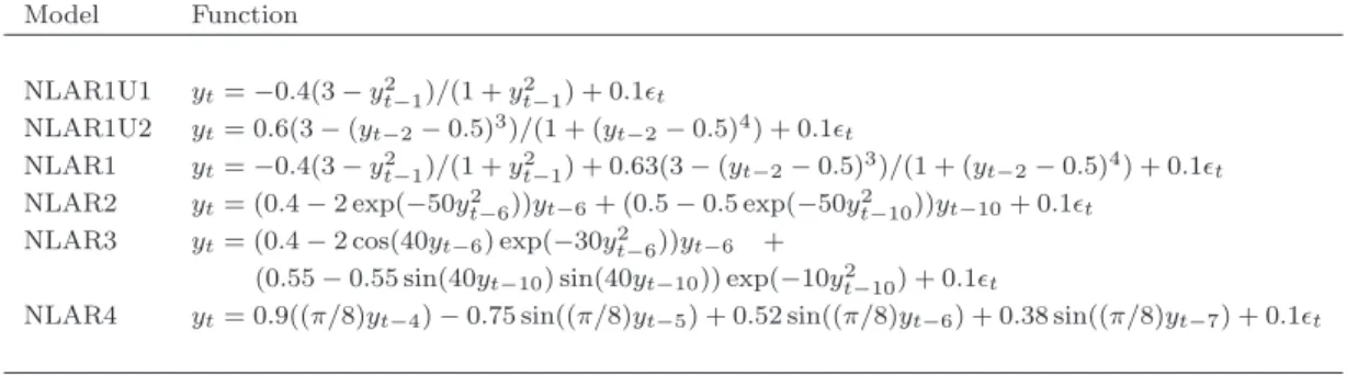
4.3 Nonlinear Autoregressive Models . . . 41
4.3.1 Spline Fitting with BIC . . . 43
4.3.2 Multivariate Adaptive Regression Splines . . . 44
4.3.3 BRUTO . . . 45
5 Simulation Study 47 5.1 Implementation . . . 47
5.2 Lag Selection . . . 49
CONTENTS CONTENTS
6 Application 56
6.1 Forecasting . . . 56
6.2 Univariate Forecasting of Industrial Production . . . 59
6.3 Forecasting with Exogenous Variables . . . 61
7 Concluding Remarks 67 Appendices 70 A APPENDIX 70 A.1 The Choice of Leading Indicators . . . 70
B APPENDIX 72 B.1 Derivation of 2.13 . . . 72
B.2 Derivation of 3.22 . . . 72
B.3 Derivation of the GLS Estimator in VAR model . . . 73
B.4 Derivation of the OLS Estimator in VAR model . . . 73
B.5 Definition of the column stacking operator vec . . . 74
C APPENDIX 75 C.1 B-Splines . . . 75
C.2 Selected Lags by GAMBoost . . . 76
C.3 Lag Functions . . . 77
C.4 Boosting Estimates of Lag Functions . . . 80
D APPENDIX: R-Code 86
1 INTRODUCTION
1
Introduction
Time series could be any sequence of data points measured at successive time in-tervals. An essential property of this sequence is its unclear evolution over time. Still, some paths remain more probable than others and this motivates researchers to try to understand the generating mechanism of the data points and possibly to forecast its future events, even before they have occurred. Linear models provide a starting point for modelling the nature of time series. Linear time series models, however, encounter various limitations in the real world and that makes them ap-plicable only under certain, very restrictive, conditions. The field of time series has undergone various new developments in the last two decades, which relaxed some of these constraints. In particular, the development of nonparametric regression added more flexibility to the standard linear regression, which was adopted by the time series paradigm as well. A leading aspect to be explored throughout the thesis is the nonparametric modelling and the resulting forecasting techniques.
The second major aspect will concern the issue of high-dimensionality in the mod-els, i.e. models with many covariates. The development of nonparametric analysis even in high dimensions was made possible thanks to the availability of suitable software and technological solutions. One of the most powerful strategies that deal with high-dimensional models comes from the machine learning community. The idea has undergone extensive evolution in the last decade and as a result, now we have available an ensemble procedure for regression under the name boosting. The novel component of the present work is the application of boosting to time series, which is done by letting the covariates be lagged values of a time series.
In the beginning of Section 2 we will explain the underlying idea of nonparametric regression through basis expansions and will emphasize how it links to linear regres-sion. We will also exemplify basis expansions through splines and will explain the real breakthrough in the nonparametric regression, obtained through the application of penalized B-Splines.
Section 3 introduces the gradient-descent view of boosting, which is considered purely as a numerical optimization, rather than as a “traditional” statistical model. We will examine the structure of several boosting algorithms for continuous data and link them to the framework of statistical estimation. We will discuss the gen-eral ideas behind componentwise boosting of linear models. We will also study two possible strategies for componentwise boosting of additive models, built on top of penalized B-Splines and will finish with discussion on the theoretical grounds behind
1 INTRODUCTION
multivariate linear boosting.
Section 4 will start with a close look of the foundation of univariate autoregressive time series analysis. We will discuss some of the aforementioned necessary con-ditions, which make the linear time series models work. Actually, even for these constrained classes of time series, as the linear autoregressive time series are, there are plenty of aspects that should be considered in order to provide a full research. Our intention is to address just the most relevant modelling principles in order to avoid overwhelming, but still provide a sound theoretical base. We will outline the relevant aspects of vector autoregressive times series models as well. The literature offers a great deal of modelling tools for nonlinear times series. Initially we will outline some of the common parametric nonlinear models, followed by an outlook of the mechanisms of the most popular nonparametric algorithms.
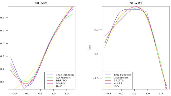
The results of a simulation study will be examined in Section 5. We will analyse the performance of boosting with P-Spline base learners in Monte Carlo simulations with six artificial, nonlinear, autoregressive time series. We will compare the outcomes of boosting to the outcomes, obtained through alternative nonparametric methods. Their performances will be considered in terms of lag-selection and goodness-of-fit. Boosting of linear and additive model will be applied to real world data in Section 6. The target variable is the German industrial production. We will compare boosting, along with other methods, to the simple univariate autoregressive model in order to answer one very appealing question: do these sophisticated techniques actually manage to outperform the linear autoregressive model in terms of forecasting? Then we will extend the data set with exogenous variables, thus building several bivariate time series. We will include the standard tool from the macroeconomic forecasting field, namely the vector autoregressive model. Finally, we will create a real high-dimensional model by including all nine exogenous variables with their respective lags into one model and will examine the forecasting performance of boosting. In Section 7 we conclude.
2 SPLINES
2
Splines
In this section we will outline basic statistical methods for nonparametric modelling through basis expansions. Basis expansions are at the heart of many nonparametric methods, presented in this thesis. Therefore, we will reveal their key concepts in order to facilitate the exposition later on. Still, other nonparametric techniques are available in Hastie and Tibshirani (1990, Chapter 2); Hastie, Tibshirani, and Fried-man (2001, Chapter 6); Fahrmeir and Tutz (2001, Chapter 5), among others. The exposition in this section will follow mainly: Eilers and Marx (1996), who made the real breakthrough in the development of splines for regression; Wood (2006), who provides a very thorough theoretical treatment and extensive material of practical application of splines, using the statistical software R (R Development Core Team, 2008); and will draw partly on Hastie et al. (2001) and Kneib (2003).
Section 2.1 will introduce the underlying idea of basis expansions and will emphasize on their connection with linear regression. In Sections 2.2 and 2.3 we will exam-ine some simple basis examples such as polynomial splexam-ines, truncated splexam-ines and B-Splines. Subsequently, we will extend them to the fundamental concept of penal-ized splines in Section 2.4, which also relates to the paradigm of additive boosting, described later in the thesis.
2.1
Basics
The most famous statistical model is the simple linear model
y=Xβ˜ +² (2.1)
where vector y = (y1, . . . , yn)T contains n realizations of the continuous response
variable y, X = (1,x1, . . . ,xp), xj = (x1j, . . . , xnj)T is the design matrix, which
summarizes an intercept and the realizations of sayppredictor variables{x1, . . . , xp},
also calledcovariates orinputs, ˜β gathers the linear impact of each covariate at the response and an error term ² = (²1, . . . , ²n)T. The notation ˜β helps us just to
distinguish these parameters from the ones in (2.5) below and implies no unusual interpretation. There are several reasons for the popularity of this model, some of them being the convenient ways of estimation the unknown parameters in ˜β. Further on, these are easily interpretable and therefore preferred from non-statisticians as well.
However, in practice it is unlikely that the random variable y and the covariates
2.1 Basics 2 SPLINES
Models (GAM) (Hastie and Tibshirani, 1990) proposes an alternative for flexible specification of the dependence through
yi =f1(xi1) +. . .+fp(xip) +²i (2.2)
wherexij, i= 1, . . . , n,is theith observation of the jth predictor and fj’s represent
smooth functions which are to be estimated instead of the parameters in ˜β. Model structures such as (2.2) represent methods for moving “beyond linearity”. The quotation marks serve to emphasize the common knowledge, that in fact, many nonlinear techniques are direct generalizations of the linear methods. The basic idea of basis expansion is to replace the inputs x1, . . . , xp by additional variables,
which are their transformations, and then use the linear methods in this new space of derived input features. This can be done by choosing a basis, defining the space of saym completely knownbasis functions. Every singlefj in (2.2) is an element of
this basis. Denote by b[jl](xij) the lth transformation of xij, then fj is assumed to
have a representation fj(xij) = m X l=1 b[jl](xij)βj[l] (2.3)
and substituting (2.3) into (2.2) yields a clear linear model
yi = m X l=1 b[1l](xi1)β1[l]+. . .+ m X l=1 b[l] p(xip)βp[l]+²i = m X l=1 p X j=1 b[jl](xij)βj[l]+²i (2.4)
The latter could be equivalently represented in a matrix notation which leads to
y=Zβ+² (2.5)
where Z = (Z1, . . . ,Zp) is the augmented (n ×mp) design matrix, Z1, . . . ,Zp are
(n×m) matrices, each representing the basis transformation of the initial vectors
x1, . . . ,xp such that Zj = (bj[1](xj), . . . , bj[m](xj)), β = (βT1, . . . ,βTp)T is a (mp×1)
parameter vector, βj = (βj[1], . . . , βj[m])T and ² is a (n×1) error vector. One easily
encounters the beauty of this approach, consisting in the similarity between (2.1) and (2.5). Once the basis functionsb[jm]have been determined, the models are linear in these new variables, and the fitting proceeds as in (2.1). Note, that interpreting the name nonparametric as absence of any parameters would be not quite precise, since β contains, indeed, very large number of parameters, which in turn have to be estimated. In order to precise the description, Eilers and Marx (1996) explain in their introduction basis expansion as an overparametric technique or equivalently
2.2 Splines 2 SPLINES
no direct statistical interpretation. Having noted this, however, we continue to follow the common concept, which describes basis expansions as a nonparametric technique.
For the sake of convenience we will restrict the number of the covariates p = 1 in the next two sections. Thus, avoiding the redundant notation (the jth index falls away) we will concentrate on the functionality of splines. Besides, the boosting algorithms presented in sections 3.2 and 3.3 imply componentwise processing with the covariates. The latter means that we are always working with one predictor at a time and therefore escape the need for simultaneous treatment of multiple predictors. This parsimony implies the following interpretation of the notation: β=β1,Z =Z1, b[l] =b[1l] and f =f1.
2.2
Splines
Splines propose a very convenient way for choosing the aforementioned basis func-tions. Before we introduce splines, we define a polynomial. Polynomial is a mathe-matical expression involving a sum of powers in one or more variables multiplied by coefficients. A polynomial spline is a curve, made up of sections of polynomials
(piecewise polynomials) joined together so that they are continuous in value, as well
as derivatives up to the degree of the polynomial minus one. These polynomials are referred to as the basis functions. The points at which the sections join are known as the knots of the spline. Typically the knots are evenly spread over the domain and are used by the spline function to connect the neighbouring polynomial pieces in a special smooth way. That means, that having knot locations denoted by τm,
a=τ1, . . . , < τM =b, S : [a, b]→R consists of polynomial pieces bi : [τi, τi+1)→R, S is said to be a polynomial spline of degree l if
1. bi has degree at most l in the subintervals [τi, τi+1)
2. S is l−1 times continuously differentiable.
A general approach to splines can be found in the books by Wahba (1990) and Gu (2002).
Given the knot locations, there are many alternatives of writing down a basis for splines. For instance, a very simple spline functionfoflth order could be represented via polynomial basis, such as:
2.2 Splines 2 SPLINES
This means that (2.3) could be written as
f(x) = β1b[1](x) +β2b[2](x) +β3b[3](x) +β4b[4](x) +. . .+βlb[m](x)
=β1+β2x+β3x2+β4x3+. . .+βmxm−1.
Another option proposes the regression spline, represented as a linear combination of a truncated power basis,
b[1](x;l) = 1, b[2](x;l) = x and b[k+2](x;l) = (x−τ k)l+, where (x−τk)l+ = (x−τk)l if x≥τk, 0 otherwise.
One could find even more complicated examples such as the one in Gu (2002, pg. 37): b[1](x) = 1, b[2](x) =x and b[k+2](x) =R(x, τk) where R(x, τk) = "µ τk− 1 2 ¶2 − 1 12 # "µ x− 1 2 ¶2 − 1 12 # /4 − "µ |x−τk| − 1 2 ¶4 − 1 2 µ |x−τk| − 1 2 ¶2 + 7 240 # /24.
However, despite the diversity of available options, all of these basis functions have one purpose, namely to map the scalarxi into theith row vector, of the augmented
matrix Z, denoted by z(i), i.e. xi 7→z(i)= £ b[1](x i), . . . , b[m](xi) ¤ .
It should be noted that in case some subinterval [τi, τi+1) is empty, that would lead
to a singular design matrix Z and consequently prevent the standard estimation process of β in (2.3). Since this it is rather unlikely to happen, we will always assume a full rank design matrix.
The proposed basis functions are relatively simple and straightforward to implement. However, they are not locally defined, which turns out to be a substantial drawback for the penalizing concept later on. A large number of knots often leads to numerical problems due to unbounded basis functions. Therefore, for regression problems we will explore one of the most convenient basis representations, namely the Basic Splines, hence B-Splines.
2.3 B-Splines 2 SPLINES
2.3
B-Splines
A primary reference for B-Splines in numerical analysis is De Boor (1978, 2001). A real breakthrough for statistics was made by Eilers and Marx (1996), who showed that penalized B-Splines are very attractive as basis functions for regression. Before we study their method in the next section, basic overview of B-Splines is proposed. The definition of the ith B-Spline basis of degree l is recursive, and namely:
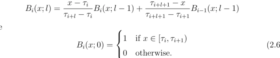
Bi(x;l) = x−τi τi+l−τi Bi(x;l−1) + τi+l+1−x τi+l+1−τi+1 Bi−1(x;l−1) where Bi(x; 0) = 1 if x∈[τi, τi+1) 0 otherwise. (2.6)
Figure 1 shows a sequence of B-Splines up to order three with evenly spaced knots from 0 to 1. The total number of knots needed for construction of k B-Splines of order l is k + 2l + 1. Note, that B-Splines of order l overlap with exactly 2l
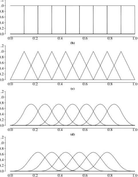
neighbours. In Figure 1, the leftmost and the rightmost splines, which have less overlap, are not depicted (see Appendix C.1, Figure 11 for the full illustration). With the assistance of the illustration in Figure 1 we could easily observe some of the appealing properties of B-Splines. Each function is nonzero over the intervals betweenl+ 2 adjacent knots, which means that the basis functions are strictly local. Moreover, in contrast to the polynomial basis, the basis functions are now bounded which leads to the numerical advantages and enhanced stability. Consider Eilers and Marx (1996) for further details on the appealing properties of B-Splines. The application of basis expansions on regression is best seen by example. In Figure 2 is shown an illustration of how B-Splines of order three, also called cubic splines, are related to the regression framework. Suppose we have an original basis of six functions, as depicted in Figure 2(a). Each function of 2(a) is multiplied by a coefficient, which results in different curves, shown in 2(b). The coefficients are usually provided by the associated parameter vector ˆβ, estimated in (2.5). For an illustration purpose, let us choose: ˆβ = (−0.2,−1.0,−0.8,1.2,0.5,0.8)T. Then, the
scaled functions from 2(b) are summed up, thus producing an estimation ˆf, depicted in 2(c).
Although B-Splines circumvent some of the major drawbacks of polynomial splines, they still require several subjective decisions in order to produce satisfying results. The first one, which is actually of minor importance, is the order of the B-Splines. The practice shows that the estimation procedure is not very sensitive to this option
2.3 B-Splines 2 SPLINES (a) 0.0 0.2 0.4 0.6 0.8 1.0 0.0 0.2 0.4 0.6 0.8 1.0 1.2 (b) 0.0 0.2 0.4 0.6 0.8 1.0 0.0 0.2 0.4 0.6 0.8 1.0 1.2 (c) 0.0 0.2 0.4 0.6 0.8 1.0 0.0 0.2 0.4 0.6 0.8 1.0 1.2 (d) 0.0 0.2 0.4 0.6 0.8 1.0 0.0 0.2 0.4 0.6 0.8 1.0 1.2
Figure 1: A sequence of B-Splines of order 0 (a), 1 (b), 2 (c) and 3(d). The leftmost and rightmost splines are discarded.
and B-Splines of order three are usually a reasonable choice. A quote of Hastie et al. (2001, p. 120) states that,
it is claimed that cubic splines are the lowest-order spline for which the
knot-discontinuity is not visible to the human eye.
The next option, however, is of major importance. It addresses the number of knots, which strongly influences the degree of smoothness. Too small number of knots leads to very smooth spline curve, which fits the data poorly. On the other hand, if the number of knots is too large the spline curve is very rough. This is a consequence of fitting the noise, as well as the underlying process. There are two common
2.3 B-Splines 2 SPLINES (a) 0.0 0.2 0.4 0.6 0.8 1.0 −1.0 −0.5 0.0 0.5 1.0 (b) 0.0 0.2 0.4 0.6 0.8 1.0 −1.0 −0.5 0.0 0.5 1.0 (c) 0.0 0.2 0.4 0.6 0.8 1.0 −1.0 −0.5 0.0 0.5 1.0
Figure 2: Nonparametric regression with B-Splines. Panel (a) depicts cubic basis functions, panel (b) shows the basis functions, multiplied by their associated coef-ficients βˆ. The sum of the scaled functions gives the spline itself, shown in panel (c).
strategies that deal with this issue. One could apply a data-driven knot selection model (Friedman and Silverman (1989); Friedman (1991); Stone et al. (1997)) or use a maximal set of knots and penalize the curvature in the estimated function. Since one of the major topics in this thesis, namely additive boosting (Sections 3.2 and 3.3) develops estimation procedure, which is based on penalized splines, we will consider the penalization concept in the following section.
2.4 P-Splines 2 SPLINES
2.4
P-Splines
Before we get familiar with the so called P-Splines (Eilers and Marx, 1996), we briefly introduce the more general form of penalized regression splines, called smoothing
splines. The appealing feature of the penalization concept is the fact that a single
parameter could control the degree of smoothness. That means that, rather than minimizing
n
X
i=1
(yi−f(xi))2
one could minimize n
X i=1 (yi−f(xi))2 +λ Z µ ∂2f ∂x2 ¶2 dx (2.7)
where f has continuous first and second derivatives, and the second derivative is quadratically integrable. The resulting estimation is called anatural cubic smoothing
spline (Reinsch, 1967). The first term in (2.7) measures the closeness to the data,
the second penalizes the curvature in f and the (tuneable) smoothing parameter λ
establishes the tradeoff between them. Ifλ = 0, then we clearly get the unpenalized estimator, which leads to a very rough function estimation. If we let λ = ∞, that would lead to the smoothest possible curve estimation, namely a straight line. It can be shown that the natural cubic smoothing spline isunique minimizer of (2.7) with knots at the values of xi (Wood, 2006, p. 148). This results in n free parameters
which are to be estimated.
Eilers and Marx (1996) propose a special form of penalized regression splines which greatly reduces the number of the parameters to estimate. They consider a discrete approximation of (2.7) with B-Splines and term it Penalized B-Splines, hence P-Splines. The main idea is that one keeps the basis dimension fixed, at a size a little larger than it is believed could reasonably be necessary (more than 30 knots do not indicate significant improvement) and penalizes directly the squared differences of the coefficients of adjacent basis functions. Moreover, the knots are evenly spaced and the recursive definition of B-Splines ensures very convenient computation of their derivatives. Thus, for any function f:
2.4 P-Splines 2 SPLINES
De Boor (1978) showed that the first derivative off could easily be calculated trough the following formula:
∂f ∂x = 1 h m X i=1 βi[Bi(x;l−1)−Bi+1(x;l−1)] = 1 h m X i=2 (βi−βi−1)Bi(x;l−1) = 1 h m X i=2 ∆βiBi(x;l−1) (2.9)
whereh denotes the distance between two adjacent knots, ∆ is the difference oper-ator, recursively defined by
∆βi =βi−βi−1
∆2β
i = ∆(∆βi) =βi−2βi−1+βi−2.
Later by induction Eilers and Marx (1996) showed that
∂2f ∂x2 = 1 h2 m X i=3 (βi−2βi−1 +βi−2)Bi(x;l−2) = 1 h2 m X i=3 ∆2β iBi(x;l−2). (2.10)
It turns out that the second term in (2.7) can be approximated in the following way:
Z µ ∂2f ∂x2 ¶2 dx= Z (D2β)TD2βdx=βTDT2D2β (2.11) where D2 = 1 −2 1 0 . 0 1 −2 1 . . . . . . . . 1 −2 1 (m−2×m)
and therefore the approximation of (2.7) can be written as
||y−Zβ||2 +λβTΛβ (2.12)
where Λ = DT2D2. Now minimizing (2.12) with respect to β, one obtains the penalized least squares estimator
ˆ
β= (ZTZ+λΛ)−1ZTy (2.13)
(see the derivation in Appendix B.1) and therefore the hat matrix (or influence
matrix) can be written as
2.4 P-Splines 2 SPLINES
The hat matrix is the one which yields the fitted vector, µ = Zβˆ = Hy, when post-multiplied by the data vector y. Moreover, it has the very useful property of determining the flexibility of the model. More precisely, the model’s flexibility is determined by the effective degrees of freedom, defined by the trace of the hat matrix. Clearly, withλset to zero the degrees of freedom of the model would be the dimension of β. At the opposite extreme, if λ is very high then the model will be quite inflexible and will hence have very few degrees of freedom, equal to the order of difference penalty.
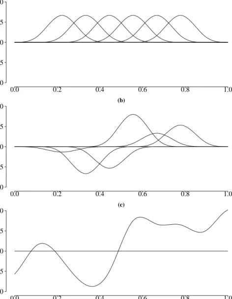
In Figure 3 are depicted three fits with different values of the smoothing parameter in order to gain a graphical impression of its impact. Ifλ is too high, then we have oversmoothing (or underfitting) and we miss the underlying dynamics of the real model. Withλ too small the data will be undersmoothed (or overfitted), describing this way too much noise. These considerations will be of use once again when we discuss boosting of an additive model in the next section. The choice of λ will be, indeed, of minor importance, since we will always provide sufficiently large value for λ and will compensate the model inflexibility through the number of boosting iterations. Despite that, for the sake of integrity we will now briefly outline some basic techniques for a proper choice of the smoothing parameter. To see this topic in a greater depth, consider for example (Wood, 2006, Chapters 3 and 4).
Generally, we find an estimation of the smoothing parameter through numerical optimization of some information criterion with respect to λ. One possibility for estimating an “ideal”λproposes theordinary cross validationscore, which estimates the expected squared error of the model. The idea consists of consecutive out-of-sample predictions of each value yi. More precisely, we leave every (xi, yi)-pair out
of the model, fit the remaining data and provide an estimation of yi, based on xi.
Finally we calculate the squared difference between the estimated and the real value of yi. Let ˆfλ[−i] denote the model fit at xi (also known as jackknifed fit atxi). Then
the formal definition of ordinary cross validation is
CV(λ) = 1 n n X i=1 ( ˆfλ[−i]−yi)2. (2.15)
Since it is inefficient to calculate n model fits, especially for large sample sizes, we could employ the hat matrix as a useful measure. It can be shown (Hastie and Tibshirani, 1990, p. 47-48) that (2.15) is equivalent to
CV(λ) = 1 n n X i=1 Ã yi−fˆλ,i 1− Hii(λ) !2 (2.16)
2.4 P-Splines 2 SPLINES 0 5 10 15 20 25 30 35 2.0 2.5 3.0 3.5 4.0 4.5 λ =100 0 5 10 15 20 25 30 35 2.0 2.5 3.0 3.5 4.0 4.5 λ =1 0 5 10 15 20 25 30 35 2.0 2.5 3.0 3.5 4.0 4.5 λ =0.01
Figure 3: Penalized regression spline fits using three different values for the smooth-ing parameter λ.
where ˆfλ,i is the ith component of the estimate, produced by fitting the full data,
and Hii(λ) are the main diagonal elements of the hat matrix. In practice, Hii(λ) is
replaced by tr(H(λ))/n which defines the Generalized Cross Validation (GCV):
GCV(λ) = 1 n n X i=1 Ã yi−fˆλ,i 1−tr(H(λ))/n !2 . (2.17)
With tr(H(λ)) we indicate the trace of the hat matrix. Thanks to its usefulness, various modelling strategies are based on slight modifications of the GCV criterion.
3 BOOSTING
3
Boosting
Boosting, as one of the most powerful ideas in the machine learning community, has been a field of increased research interest in the last decade. Real breakthrough for a two class problem, i.e. response y ∈ {1,0}, was made by Freund and Schapire (1996) with their AdaBoost algorithm.
Later Breiman (1996) provides experimental and theoretical evidence that his method “bootstrapaggregating”, hence bagging, can give substantial improvement in accu-racy for both classification and regression prediction. Although unstable in predic-tion, his method makes a significant step towards optimality, by incorporating the idea of generating multiple versions of a predictor and then producing an aggregated predictor by plurality vote. A “committee” based approach is the basic concept of boosting as well. Breiman (1998) noted that the AdaBoost algorithm can be consid-ered as a gradient descent optimization technique in function space. These findings opened perspective to consider boosting for regression problems which was success-fully developed later by Friedman (2001). In the context of regression, the gradient boosting proposed by Friedman is essentially the same as Mallat and Zhang’s (1993) matching pursuit algorithm in signal processing.
3.1
Gradient Boosting
3.1.1 Steepest Descent
The statistical framework developed by Friedman (2001) interprets boosting as a method for direct function estimation. He showed that boosting could be inter-preted as a basis expansion, in which every single basis term is iteratively defined by the preceding ones. Suppose we have a random output variable y and a set of explanatory or input variablesx= (x1, . . . , xp) the goal is, using a “training” sample
{yi,x(i)}n1, wherex(i)∈Rp is ap-dimensional row-vector, to obtain an estimate ˆf(x)
of the function f(x), which maps xto y. To achieve this approximation one has to specify a loss functionL(y, f), and to minimize the expectation of this loss function with respect to f. A discussion about the specification of several loss functions follows in Section 3.1.2 below. The minimization off can be viewed as a numerical optimization problem such as
ˆ f = arg min f L(y, f) (3.1) where L(y, f) = n X i=1 L(yi, f(x(i))). (3.2)
3.1 Gradient Boosting 3 BOOSTING
A common procedure that solves (3.1) is to restrict f(x) to be a member of a parameterized class of functions f(x;θ). For instance, f(x;θ) can be viewed as an additive expansion of the form
f(x;β,γ) =
M
X
m=1
βmh(x;γm)
where the basis function h(x;γ) is characterized by a set of parameters γ, i.e. the members of this expansion differ in the parameters γm. Thus, the originalfunction
optimization problem has been changed to aparameter optimization problem. That is, optimize {βˆ,γˆ}= arg min β,γ n X i=1 L(yi, f(x(i);β,γ)) (3.3) in order to achieve ˆ f =f(x; ˆβ,γ)ˆ . (3.4)
In many situations, however, it is unfeasible to solve (3.3) directly and therefore an alternative numerical optimization method should be applied. One possibility is to try agreedy stagewise approach, which is
{βm,γm}= arg minβ,γ n X i=1 L(yi, fm−1(x(i)) +β h(x(i);γ)) (3.5) followed by fm(x) = fm−1(x) +βmh(x;γm). (3.6)
In machine learning a strategy like the sequence (3.5)-(3.6) is called boosting and the function h(x;γ) is termed a weak learner or a base learner. There are various modifications of the boosting strategy, differing mostly in the base learner. We will examine some of them in the following sections. However, the solution of (3.5) is not always feasible and requires a numerical optimization method itself. One such method is the steepest-descent optimization algorithm. Given any approximation
fm−1(x), the increments βmh(x;γm) in (3.5)-(3.6) are determined by computing
the current gradient:
−gm(x(i)) = · ∂L(yi, f(x(i))) ∂f(x(i)) ¸ f(x)=fm−1(x) (3.7) which gives the steepest-descent direction −gm =−(gm(x(1)), . . . , gm(x(n)))T ∈Rn.
Note, that the gradient is defined only at the training data points and cannot be gen-eralized to otherx-values. If the only goal was to minimize the loss on the training data the “steepest descent” would be sufficient. One possibility for generalization to new data, not presented in the training set, is to choose thath(x;γ) which produces
3.1 Gradient Boosting 3 BOOSTING hm = (h(x(1);γm), . . . , h(x(n);γm))T most parallel to the gradient −gm, i.e. this
h(x;γ), which is most highly correlated with the gradient −g(x). This can be done simply by fitting h(x;γ) to the “pseudoresponse” −g(x), i.e.
γm = arg min β,γ n X i=1 (−gm(x(i))−β h(x(i);γ))2. (3.8)
Furthermore, a more powerful strategy would be to multiply the gradient vector with some constant in order to go into a “better” direction, which is called line search.1 That means that we additionally compute
ρm = arg min ρ n X i=1 L(yi, fm−1(x(i)) +ρ h(x(i);γm)) (3.9)
and finally the updates are determined via
fm(x) =fm−1(x) +ρmh(x; ˆγm).
Now we summarize steepest descent boosting as the following generic algorithm:
Generic Gradient Descent Boosting 1. Initialize f0 = arg minρ
Pn i=1L(yi, ρ), m= 0 2. m=m+ 1 3. ri =− h ∂L(yi,f(x(i))) ∂f(x(i)) i f(x)=fm−1(x) , i= 1, . . . , n 4. γm = arg minβ,γ Pn i=1(ri−β h(x(i);γ))2 5. ρm = arg minρ Pn i=1L(yi, fm−1(x(i)) +ρ h(x(i);γm)) 6. fm(x) = fm−1(x) +ρmh(x;γm) 7. Iterate 2-6 untilm=M
where the best value for M can be obtained via cross-validation.
3.1.2 Loss Functions
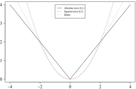
Expression (3.7) hints at the importance of the prechosen loss function. In addition to the weak learner, this is the second major option which determines the nature of the generic algorithm. Therefore several options for choosing the loss are briefly discussed in the sequel.
One of the frequently employed loss functions L(y, f(x)) is the squared-error loss,
1It should be noted that the line search can be automatically provided through β when
3.1 Gradient Boosting 3 BOOSTING −4 −2 0 2 4 0 1 2 3 4 y − f Loss Absolute error (L1) Squared error (L2) Huber
Figure 4: A comparison of three loss functions for regression, plotted as a function of y−f(x).
also called L2-loss, L(y, f(x)) = 1
2(y− f(x))2. It is scaled by the factor 12 thus
ensuring a convenient representation of its first derivative (simply the residuals) which becomes very useful at line 3 of the generic algorithm. An absolute-error lossL(y, f(x)) = |y−f(x)| orL1-loss is another famous example for loss criterion. Although not differentiable at the points yi =f(x(i)), partial derivatives of L1-loss
could be computed due to the zero probability of realizing single pointyi =f(x(i)) by
the data. The last one to examine is the Huber loss criterion used for M-regression (Huber, 1964) and defined as:
L(y, f(x)) = |y−f(x)|2/2 if |y−f(x)| ≤δ, δ(|y−f(x)| −δ/2) if |y−f(x)|> δ
where a strategy for adaptively changing δ is proposed by Friedman (2001):
δm = median ({|yi −fm−1(x(i))|; i= 1, . . . , n}).
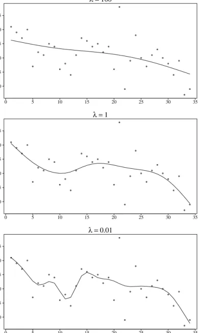
Figure 4 proposes a graphical interpretation of the loss functions. The squared-error loss penalizes observations with large absolute residuals more heavily than the other two criteria. Thus L2-loss is far less robust and its performance degrades for
dis-tributions with heavy tails and especially by presence of outliers. L1-loss penalizes
the extreme margins only linearly and thus Huber-loss is somewhat a compromise between them.
3.1 Gradient Boosting 3 BOOSTING
Furthermore, a very convenient property is the computational simplicity of the gra-dients of these loss functions. The loss criteria and the corresponding gragra-dients are summarized in Table 1. Recall the generic gradient boosting strategy. Applied
Loss Function ∂L(y, f(x))/∂f(x)
L1 sign{y−f(x)}
L2 y−f(x)
Huber y−f(x) for |y−f(x)| ≤δm
δm sign{y−f(x)} for |y−f(x)|> δm
Table 1: Gradients for commonly used loss funcitons.
to the most popular L2-loss, it turns out that Least Squares Boosting (LS Boost,
Friedman (2001)) is nothing more than repeated least squares fitting of residuals (see line 4 of the generic gradient descent boosting). Furthermore, line 5 (the line search) is not needed anymore because ρm = βm and βm was computed already at
line 4. Essentially the same procedure with M = 2 has been proposed by Tukey (1977) and termed “twicing”. Gradient boosting with squared-error loss produces the following algorithm:
LS Boost 1. f0(x) = ¯y, m = 0 2. m =m+ 1 3. ri =yi−fm−1(x(i)), i= 1, . . . , n 4. (βm,γm) = arg minβ,γ Pn i=1(ri−β h(xi;γ))2 5. fm(x) =fm−1(x) +βmh(x;γm) 6. Iterate 2-5 untilm =M
where the best value for M is usually determined via cross-validation.
3.1.3 Regularization
One virtual problem of prediction is encountered, when the training data is fitted too closely. This hinders the good prediction when working with new data and is calledoverfitting. The impressive performance of boosting is mainly due to its resis-tance to overfitting. Initially, this appealing property was observed empirically, until B¨uhlmann and Yu (2003) provided an analytical proof. The key to this resistance comes at the price of one extra parameter introduced by a regularization method
3.1 Gradient Boosting 3 BOOSTING
called shrinkage. It attempts to prevent overfitting by constraining the fitting pro-cedure with a shrinkage factor. The simple strategy is to replace line 6 of the generic algorithm (respectively line 5 of the LS Boost) with
fm(x) =fm−1(x) +ν ρmh(x;γm) (3.10)
where ν is the shrinkage factor. On the other hand, as the boosting iterations evolve, the estimation model has more terms which suggests the “natural” way of overfit prevention - providing small number of covariates, i.e. small M. It turns out that we have two instruments for prevention which work in different manners. Regularizing by controlling the number of influence terms suggests that “sparse” ap-proximations, i.e. models which involve fewer terms, are believed to provide better prediction. However, it has often been found that regularization through shrinkage provides superior results to that obtained by restricting the number of covariates. The shrinkage can be regarded as controlling the learning rate of the boosting proce-dure. Roughly speaking, it provides the weak learner to be “weak” enough, i.e. the base learner has large bias but low variance. Nevertheless, these parameters do not operate independently and therefore mutually affect their performances. Decreasing the values of ν increases the best value for M, so there is a tradeoff between them. Ideally one should estimate optimal values for both by minimizing a model selection criterion jointly with respect to the values of both parameters. The performance of
ν is examined rather empirically and Friedman (2001) was the first to demonstrate that small values (ν = 0.3) are good in sense of low sensitivity of the boosting procedure.
3.1.4 Boosting with Linear Operator
B¨uhlmann and Yu (2003) made the next significant contribution to the intensively developing boosting framework. Their work contributed in several aspects, most notably: they proposed a learner via linear operatorS, which was appropriately ad-justed later for the componentwise approach; they managed to prove an exponential dependence between the bias and the variance of the boosted model, which is the reason for the overfit resistane2 of boosting; they showed how smoothing splines can
be adopted by the boosting base procedure. In this section we will consider the first aspect.
Roughly speaking, the key idea is to represent the learner as a linear operator (or
smoother) S : Rn → Rn, which yields the fitted values when post-multiplied by
2It was shown that addition of new terms in the model does not linearly increase its complexity,
3.2 Boosting High-Dimensional Models 3 BOOSTING
the pseudo response. Let us denote hm = (βmh(x(1);γm), . . . , βmh(x(n);γm))T,
fm = (fm(x(1)), . . . , fm(x(n)))T, y= (y1, . . . , yn)T and rm =y−fm−1. Furthermore
we use the basic relation from the generic boosting algorithm fm =fm−1+hm with
hm =Srm to provide the relationship
rm =y−fm−2− Srm−1
=rm−1− Srm−1.
Since f0 =Sy, then follows r1 = (I − S)y and we obtain
rm = (I− S)my. (3.11)
Consequently
fm =y−rm+1 = (I −(I − S)m+1)y
and finally the operator that maps the initial response vector y to fm is termed
Boosting operator, that is
Bm =I−(I− S)m+1. (3.12)
Expression (3.12) enables us to define the presence of “learning capacity” of the model such that kI − Sk < 1. In addition, Bm converges to the identity I as
m → ∞, thereby Bmy converges to the fully saturated model y, interpolating the
response exactly. However, using the same smoother S still does not explicitly suggest variable selection and is therefore best applicable for univariate problems. In the following Section 3.2 we will shown how this flexibility can be adopted by boosting even for high-dimensional models, where the number of predictor variables is allowed to grow very quickly.
3.2
Boosting High-Dimensional Models
B¨uhlmann (2006) provided an essential boosting technique, called L2Boost, for
re-gression problems with rapidly growing number of predictor variables. The key idea in his method is to exercise the weak learner upon one variable at a time and to pick out only those components with the “largest contribution to the fit”. That is another way of keeping the learner “weak” enough, i.e. having low variance relative to the bias, which is done simply by restraining of a complex structure with many parameters. Thus, he also manages to incorporate an original predictor selection stage into the boosting paradigm. The arbitration of the model’s complexity is another distinctive feature of the new boosting technique. This complexity has an essential role for defining the stopping condition of boosting. It is not required to
3.2 Boosting High-Dimensional Models 3 BOOSTING
run the algorithm multiple times for cross-validation, as commonly used by then. A derivation of the hat matrix is provided and the complexity is determined by its trace. Using that trace, one employs a corrected version of an AIC (Hurvich, Si-monoff, and Tsai, 1998) to define the stopping criterion for the boosting algorithm. These novelties are illustrated in the sequel.
3.2.1 Componentwise Linear L2Boost
We consider a linear model with p covariates, x1, . . . , xp and a response variable y,
with xj denoting a n-dimensional vector with realizations of xj, and xkj the kth
element of this vector. The essential modification of the new strategy concerns the base learner, which is forced to docomponentwise selection among the predictors at each boosting stage. The base learner h(x) works as follows:
Componentwise linear least squares learner h(xˆs) = ˆβˆsxˆs ˆ βj = (xj −x¯j)Tr (xj −x¯j)T(xj −¯xj) , j = 1, . . . , p ˆ s= arg min 1≤j≤p n X i=1 (ri−βˆjxij)2 (3.13)
wherer= (r1, . . . , rn)T is the gradient of the loss function, used as a pseudo response.
Thus, the base procedure fits a simple linear regression with every single covariate and selects the one that reduces the residual sums of squares most. So we have a “built-in” predictor selection procedure. Finally, the L2Boost algorithm can be
summarised in the following scheme:
Componentwise boosting of linear model 1. Initialize f0 = ¯y1, set m= 0. 2. m =m+ 1 3. rm =y−fm−1 4. Find ˆsm as in (3.13). 5. Update fm =fm−1+νh(xsˆm). 6. Iterate 2-5 untilm=M
where ν is the shrinkage parameter and should accordingly be kept small, e.g. ν = 0.1, 1 = (1, . . . ,1)T and h(x
ˆ
sm) = (h(x1,ˆsm), . . . , h(xn,sˆm))
3.2 Boosting High-Dimensional Models 3 BOOSTING
structure in (5), the final estimate can again be interpreted as an additive model, but the componentwise selection suggests that it typically depends on a subset of the originalp covariates.
Unlike the common practice in gradient boosting, the stopping condition M for
L2Boost is determined via the computationally more efficient AICc information
criterion (3.17) defined below. The first requirement for providing this criterion is to determine the model complexity. Therefore, we assign degrees of freedom for boosting. Denote by
H(j) = xjxTj
kxjk2
, j = 1, . . . , p (3.14) the (n×n) hat matrix for the linear squares fitting operator using thejth predictor. It acts similarly to the linear operator S in Section 3.1.4 but employs each time different covariate. The denominator kxjk2 denotes the Euclidean norm for a n
-dimensional vector. Recall the common knowledge that the hat matrix yields the fitted vector when post-multiplied by the (pseudo) response vector, i.e. h(xsˆm) =
H(ˆsm)r
m. Moreover rm =y−fm−1 and fm =fm−1+νh(xˆsm) which is followed by
rm =y−fm−2−νH(ˆsm−1)rm−1 =rm−1−νH(ˆsm−1)rm−1 and we have rm = (I−νH(ˆsm−1)). . .(I −νH(ˆs2))(I−νH(ˆs1))y. (3.15) Then fm =y−rm+1 = (I−(I−νH(ˆsm)). . .(I −νH(ˆs1)))y
and finally theL2Boost hat matrix at stage m equals
H(m) =I−(I−νH(ˆsm)). . .(I−νH(ˆs2))(I−νH(ˆs1)). (3.16)
Note that H(ˆs) and H(
m) are hat matrices in different regression problems, i.e. H(ˆs)
maps the pseudo response while H(m) maps the initial response. The L2Boost hat
matrix H(m) ultimately depends upon the selected components ˆs1, . . . ,ˆsm. This is
a direct consequence of the componentwise approach. Therefore, the term “hat matrix” is in someway liberally transferred to H(m) and more precisely should be
viewed as an approximate hat matrix. Conversely, the Boosting operator (3.12) uses the same operator (or smoother) at every stage, thus excluding the componentwise fashion of modelling.
3.2 Boosting High-Dimensional Models 3 BOOSTING
version of AIC in order to define a stopping condition for boosting:
AICc(m) = log(ˆσ2) + 1 + tr(H(m))/n (1−tr(H(m)) + 2)/n (3.17) ˆ σ2 =n−1 n X i=1 (yi−(Hmy)i)2.
The number of boosting iterations is then estimated ˆ
M = arg min
1≤m≤MAICc(m)
where M is large enough to be used as an upper bound for the candidate number of iterations.
3.2.2 Componentwise Additive L2Boost
The final remarks in Section 3.1.4 suggested the possibility of adding a nonparamet-ric procedure to the boosting framework. Therefore, we assume additive expansion3
of the predictors. In this case, a smooth function is fitted to the negative gradient of the loss function in each iteration, i.e. the parametric least squares learner from the previous section is simply substituted by its “nonparametric” (or overparamet-ric) counterpart. B¨uhlmann and Yu (2003) have shown that choosing smoothing splines as a base procedure is very competitive to standard nonparametric models. Later, Schmid and Hothorn (2007) investigated whether boosting with smoothing spline base learners can be successfully approximated by boosting with P-Spline base learners.4 Similarly to regression, it turned out that P-Splines, which are more
advantageous from a computational point of view, propose very good approximation of smoothing splines. Recall that Z1, . . . ,Zp represent the basis transformations of
the initial covariates x1, . . . ,xp such that Zj = (b[1]j (xj), . . . , b[jB](xj)) is a (n×B)
matrix. Then we have
h(xs) = Zsβs. (3.18)
Consequentlyβs is estimated via penalized least squares estimator as in (2.13). The base procedure is then:
Componentwise P-Splines as base procedure
3Note that the term additive expansion can be used in two different contexts. Here we suggest
an initial additive expansion of the covariates, which should be clearly distinguished from the interpretation of theboosting iterations as additive expansions themselves.
4We will briefly discuss in the next section the use of P-Spline base learners in an
alterna-tive boosting procedure, calledlikelihood boosting (Tutz and Binder, 2006), and show when both strategies coincide.
3.3 Likelihood Boosting 3 BOOSTING h(xˆs) =Zˆsβˆˆs ˆ βj = (ZT jZj+λΛ)−1ZTjr, j = 1, . . . , p ˆ s= arg min 1≤j≤pkr−h(xj)k (3.19)
where Λ is the penalty matrix.
The inevitable price that we pay for increased flexibility consists of additional pa-rameters. Now we should choose not only an appropriate shrinkage factorν, but also smoothing parameter λ and number of evenly spaced knots. Schmid and Hothorn (2007) carried out a thorough analysis of the effect of the various parameters on the boosting fit and provided very intriguing conclusions. They proved an approx-imately linear dependence between the number of the boosting iterations and ν
for regression with one-dimensional covariate and found empirical evidence that the same relationship also holds true for higher dimensions. This implies that theAICc
criterion (3.17) automatically adapts the stopping value for the iterations to the shrinkage factor.
Furthermore, note thatλdetermines the degrees of freedom (df) of the base learner. High values of λ lead to low degrees of freedom which is preferable in order to keep the learner “weak”. Roughly speaking, λ acts like the shrinkage factor above by reducing the learning rate of the base procedure. It was proposed by Schmid and Hothorn (2007) df = 3−4 as a suitable amount for the degrees of freedom. Their results, concerning the number of knots confirmed the common knowledge that there is a minimum number of necessary knots which have to be provided and the algo-rithm is not sensitive to this choice (20-50 knots should be sufficient). Finally, the insertion of the new learner in the boosting paradigm is rather straightforward.
3.3
Likelihood Boosting
Likelihood boosting, proposed by Tutz and Binder (2006), retains the especially useful “built-in” selection feature for high-dimensional models. Besides, it manages to generalize the “boosts” for a response following a simple exponential family like binomial, poisson or Gaussian. This is done by maximizing the likelihood in gen-eralized additive models for all kinds of link functions. The procedure is referred to as GAMBoost. One of the most advantageous innovations in GAMBoost is the relation of the Newton-Raphson method to boosting. It also restrains the explicit usage of the proposed loss functions by incorporating an information AIC criterion instead. AIC is additionally used as stopping condition.
Gen-3.3 Likelihood Boosting 3 BOOSTING
eralized Linear Models (GLM). A GLM (Nelder and Wedderburn, 1972) allows for the response distributions other than normal and has a basic structure
µi =h(ηi) =h(x(i)β) (3.20)
instead of the linear predictor
µi =ηi =x(i)β
wherex(i) is ap-dimensional predictor vector, µi = E (yi|x(i)) andhis a specified
re-sponse function. General assumptions foryi’s are their independence and belonging
to some exponential family, i.e.
fθ(y) = exp{(yθ−b(θ))/a(φ) +c(y, φ)}
whereθ is a canonical parameter which completely depends on β, φ is an arbitrary dispersion parameter and a, b and c are arbitrary functions. The log likelihood of
θ, given a particular y, is the log(fθ(yi)) considered as a function of θ and not of y
anymore. Furthermore the log likelihood of θ defines ultimately the log likelihood of β, that is l(β) = n X i=1 log(fθi(yi)) = n X i=1 (yiθi−b(θi))/a(φ) +c(φ, yi). (3.21)
Unfortunately, if the response is not Gaussian, there is no solution in closed form for (3.21), i.e. it demands numerical optimization methods such as Iteratively Re-weighted Least Squares (IRLS) or the Newthon-Raphson method. In combination with an additive structure in the covariates, fitting of model (3.21) is based on maximizing the penalized likelihood
l(p) =l(β)− λ
2Λβ.
At this stage a modified version of the Newton-Raphson method should be applied to obtain an estimation of β. It is done via the so called penalized score function
sp(β) =s(β)−λΛβ, where
s(β) =ZTjD(β)Σ(β)−1(y−µ) =ZTjW(β)D(β)−1(y−µ) with
ZT
j = (z1j, . . . ,znj) the augmented design matrix,
µ= (µ1, . . . , µn)T, ηi = ˆη(m)(x(i)) +zTijβj, D(β) = ∂h(η1)/∂η . . . . .. . . . ∂h(ηn)/∂η
3.3 Likelihood Boosting 3 BOOSTING Σ(β) = σ1 . . . . .. . . . σn σ2i = Varβ(yi), W(β) =D(β)Σ(β)−1D(β).
The penalized Fisher matrix
Fp(β) = E µ −∂2l p(β) ∂β∂βT 
has the form Fp =F(β) +λΛ, where F(β) = E
¡
−∂2l(β)/∂β∂βT¢ =ZT
jW(β)Zj.
One Fisher scoring step is then ˆ
βnew= ˆβ+Fp(ˆβ)−1sp(ˆβ)
and starting with an initial guess β(0) the solution is found through successive im-provements of β. Since with boosting one successively corrects the already fitted terms, at this stage we observe the most innovative feature of GAMBoost. Likelihood boosting requires only one step of the Fisher scoring algorithm and the estimations
ˆ
βnew are derived simply by refitting the residuals. For further details see Tutz and Binder (2006).
Assuming the special case of a Gaussian response, the notation is consistent with Section 2.1: f = µ = Zβ, whereˆ Z = (Z1, . . . ,Zp) is the augmented (n × Bp)
design matrix, Z1, . . . ,Zp represent the basis transformations of the initial
covari-ates x1, . . . ,xp, such that Zj = (b[1]j (xj), . . . , bj[B](xj)), βˆ = (βT1, . . . ,βTp)T is a
(Bp×1) vector, βj = (βj[1], . . . , βj[B])T. The weak learner is essentially the same
as in the previous section. Then, the updates of βˆ are introduced through βˆ(m) =
ˆ
β(m−1)+ (0T, . . . ,βˆT
ˆ
sm, . . . ,0
T)T, where 1≤sˆ
m ≤p denotes the fitted component at
the mth step and 0 denotes zero vectors that supplement the second addend to a conformable argument. That leads to the well-known structure
fm =Z ˆβ(m−1)+Zˆsmβˆsˆm =Z ˆβ(m) =fm−1+hm.
To stop the boosting iterations one could profit again from the sophisticated hat matrix at step k, H(k) and particularly from its ability to express the model
com-plexity by the effective degrees of freedom stuck in its trace. The hat matrix has the form H(ˆsm)= m X j=0 H(ˆsj) j−1 Y i=0 (I− H(ˆsi)) (3.22)
(see the derivation in Appendix B). Thus, in the special case of Gaussian response, additive learner and L2-loss function, the hat matrices (3.16) and (3.22) coincide.
3.4 Multivariate Boosting 3 BOOSTING
3.4
Multivariate Boosting
Allowing high dimensionality for the response in a boosting strategy has been con-sidered, up to my knowledge, only in Lutz and B¨uhlmann (2006) . They present theoretical treatment of the multivariate boosting and also provide empirical evi-dence that the multivariate approach outperforms individual estimations in several cases. Their technique strongly resembles theL2 Boosting scheme from Section 3.2, hence only the most distinctive features are outlined in the sequel. It should be noted, that this more advanced way of boosting was still not implemented in the standard add-on package mboost (Hothorn et al., 2008) at the time of writing this thesis.
A multivariate linear regression model withn observations is considered as follows:
Y =XB+E (3.23)
with Y ∈ Rn×q, X ∈ Rn×p, B ∈ Rp×q and E ∈ Rn×q. The increase of
dimension-ality demands a richer nomenclature. Therefore y(i) denotes the response at the
ith sample point, i.e. a q-dimensional row-vector. With yj is indicated the jth re-sponse variable, i.e. an-dimensional column-vector. For the error matrix is assumed E (ej) = 0, cov(e(k), e(l)) = 0, for k 6=l, that is the sample points are independent,
cov(ei) = Σ. Additionally it is assumed that all covariates are centered to have zero
mean, so no intercepts are worrying. The corresponding loss function is then
L(B) = 1 2 n X i=1 (yT (i)−xT(i)B)Γ−1(yT(i)−xT(i)B)T (3.24)
where Γ is an estimate of the usually unknown covariance matrix Σ. The well known componentwise procedure is affected by the new dimensionality in the pseudo response as well. It consistently follows the dimensionality of the initial response and is termeed with R∈ Rn×q. The componentwise learner selects again only that
component which reduces the loss function most:
Multivariate linear learner
H(xsˆ) =xsˆβˆˆs,ˆt ˆ βjk = Pq v=1RTvxjΓ−1vk xT jxjΓ−kk1 (ˆs,ˆt) = arg max 1≤j≤p,1≤k≤q ¡Pq v=1RTvxjΓ−1vk ¢2 xT jxjΓ−1kk (3.25)
3.4 Multivariate Boosting 3 BOOSTING
From (3.25) we see the impact of the multivariate structure in ˆβjk, which is not
influenced only by thekth response but also by other response-components via Γ−1
and their correlation with the jth predictor xj. The other key definition is the hat
matrix, that maps the single components to the response. That is
H(jk)= 0 0 . . . 0 ... ... ... 0 0 . . . 0 HjΓ−1k1 Γ−1 kk H jΓ−1k2 Γ−1 kk . . . H jΓ−1kg Γ−1 kk 0 0 . . . 0 ... ... ... 0 0 . . . 0 (3.26) where Hj = x
jxTj/xTjxj is the hat matrix of the univariate componentwise linear
learner using the jth predictor. Then the approximate hat matrix of the boosting at stepm is
Km =I−(I−νH(ˆsmˆtm))(I−νH(ˆsm−1tˆm−1)). . .(I−νH(ˆs1ˆt1)). (3.27)
Lutz and B¨uhlmann (2006) also provide the computational complexity of the hat matrix O(n2p+n3q2m) and conclude that such computations are not feasible for
large n orq. Finally, the stopping criterion should also be conformable with higher dimensions, which leads to
AICc(m) = log(|Σˆ(m)|) +
q(n+ trace(Km)/q)
n−trace(Km)/q−q−1
where Σˆ(m) = n−1Pn
i=1(R(i)RT(i)) and the number of boosting operations is
esti-mated via
ˆ
M = arg min
0≤m≤MAICc(m)
with a pre-chosen, sufficiently large value of M.
Alternatively, one could approach the multivariate structure by row-boosting. The concept of row-boosting is to update a whole row of B, instead of a single entry. This strategy is supported by the assumption that a single covariate could influence all response-components. The variable, which contributes to the multivariate fit most, is updated at the corresponding step. The multivariate fit is determined via Wilk’s Λ,
Λ = |(Y−XB)ˆ
T(Y−XB)ˆ |
|YTY|
3.4 Multivariate Boosting 3 BOOSTING
Lutz and B¨uhlmann (2006) showed with simulated data that multivariate boosting performs well, particularly in those situations, where the predictor dimension or the response dimension is large relative to the sample size. Row-boosting does not seem to outperform multivariate boosting, except of the situations with row-completeB. In case of correlated errors, multivariate boosting is clearly superior to the individual
L2 Boosting and at least as good with uncorrelated errors. Apparently, on real data none of the boosting techniques proves to be the overall best method. For further details see the cited paper.