HAL Id: hal-02335148
https://hal-amu.archives-ouvertes.fr/hal-02335148
Submitted on 28 Oct 2019
HAL
is a multi-disciplinary open access
archive for the deposit and dissemination of
sci-entific research documents, whether they are
pub-lished or not. The documents may come from
teaching and research institutions in France or
abroad, or from public or private research centers.
L’archive ouverte pluridisciplinaire
HAL, est
destinée au dépôt et à la diffusion de documents
scientifiques de niveau recherche, publiés ou non,
émanant des établissements d’enseignement et de
recherche français ou étrangers, des laboratoires
publics ou privés.
Distributed under a Creative Commons
Attribution| 4.0 International License
Histogram-Based Features Selection and Volume of
Interest Ranking for Brain PET Image Classification
Imene Garali, Mouloud Adel, Salah Bourennane, Eric Guedj
To cite this version:
Imene Garali, Mouloud Adel, Salah Bourennane, Eric Guedj. REHABILITATION DEVICES AND
SYSTEMS Histogram-Based Features Selection and Volume of Interest Ranking for Brain PET Image
Classification. IEEE Journal of Translational Engineering in Health and Medicine, IEEE, 2018, 6,
pp.2100212. �10.1109/JTEHM.2018.2796600�. �hal-02335148�
Received 1 June 2017; revised 3 October 2017 and 23 November 2017; accepted 27 December 2017. Date of publication 16 March 2018; date of current version 28 March 2018.
Digital Object Identifier 10.1109/JTEHM.2018.2796600
Histogram-Based Features Selection and Volume
of Interest Ranking for Brain PET
Image Classification
IMÈNE GARALI1,2, MOULOUD ADEL 1, SALAH BOURENNANE3, AND ERIC GUEDJ2,4
1Aix Marseille Univ, CNRS, Centrale Marseille, Institut Fresnel, F-13013 Marseille, France 2Institut de Neurosciences de la Timone UMR-CNRS 7289, Aix-Marseille Université, 13385 Marseille, France
3Ecole Centrale Marseille, Institut Fresnel UMR-CNRS 7249, 13013 Marseille, France
4Centre Européen de Recherche en Imagerie Médicale, Faculté de Médecine, Aix-Marseille Université, 13385 Marseille, France CORRESPONDING AUTHOR: M. ADEL ([email protected])
This work was supported in part by DHU-Imaging through the A∗MIDEX Project funded by the‘‘Investissements d’Avenir’’French
Government Program and managed by the French National Research Agency under Grant ANR-11-IDEX-0001-02, in part by the region PACA, and in part by Nicesoft.
ABSTRACT Positron emission tomography (PET) is a molecular medical imaging modality which is
commonly used for neurodegenerative diseases diagnosis. Computer-aided diagnosis, based on medical image analysis, could help quantitative evaluation of brain diseases such as Alzheimer’s disease (AD). A novel method of ranking the effectiveness of brain volume of interest (VOI) to separate healthy control from AD brains PET images is presented in this paper. Brain images are first mapped into anatomical VOIs using an atlas. Histogram-based features are then extracted and used to select and rank VOIs according to the area under curve (AUC) parameter, which produces a hierarchy of the ability of VOIs to separate between groups of subjects. The top-ranked VOIs are then input into a support vector machine classifier. The developed method is evaluated on a local database image and compared to the known selection feature methods. Results show that using AUC outperforms classification results in the case of a two group separation.
INDEX TERMS Machine learning, computer-aided diagnosis, first order statistics, feature selection, positron emission tomography, classification, Alzheimer’s disease.
I. INTRODUCTION
Alzheimer Disease (AD) is a degenerative and incurable brain disease which is considered the main cause of dementia in elderly people worldwide. It is expected that 1 in 85 people will be affected by 2050 and the number of affected people will double in the next decades [1]. The diagnosis of this disease is done by clinical, neuroimaging and neuropsycho-logical assessments. Neuroimaging evaluation is based on nonspecific features such as cerebral atrophy, which appears very late in the progression of the disease. Therefore, devel-oping new approaches for early and specific recognition of AD is of crucial importance.
Several imaging biomarkers to identify AD are effec-tive [2], including structural Magnetic Resonance Imag-ing (MRI) [3]–[7], SImag-ingle Photon Emission Computed Tomography (SPECT) [8], electroencephalographic EEG rhythms [9], [10] and Positron Emission Tomography (PET) [11], [12]. In addition to these imaging bio-markers, biological biomarkers such as Cerebral Spinal
Fluid (CSF) [6] have also been developed for AD diagno-sis. It has been shown that PET functional imaging asso-ciated with FluoroDeoxyGlucose (18F-FDG) as a tracer is able to increase the confidence of neurodegenerative diagnosis [13]–[16].
Early detection of AD is important because it increases the chances of early treatment and may enable pre-emptive and even preventative therapies in the future.
The clinical diagnosis of AD uses a variety of tests including patient’s family history, physical examination, mini-mental state examination, and/or neuroimaging [17]. Recently, functional neuroimaging technologies, such as the Positron Emission Tomography (PET), has become a powerful tools in the diagnosis of AD since it is now possible to reveal pathophysiological changes before irreversible anatomical changes are present. 18F-Fluoro-deoxyglucose (FDG) is a widely used radioactive tracer in PET imaging. FDG-PET provides useful information about the cerebral glucose metabolic rate.
2100212
2168-23722018 IEEE. Translations and content mining are permitted for academic research only. Personal use is also permitted, but republication/redistribution requires IEEE permission.
Studies have demonstrated reduced glucose metabolism in a small number of brain regions in AD patients comparing to normal subjects [18], [19]. As such difference becomes noticeable, researchers are increasingly interested in distin-guishing AD patients from normal subjects by utilizing their brain images. As a non-negligible complementary way in the diagnosis of AD, PET imaging has high specificity and sensitivity, even a long period before the full-blown dementia has developed.
Visual evaluation of brain PET images is qualitative and deals with two problems: it is time consuming and opera-tor dependent [20]. Visual method depends greatly on the observer’s experience and lacks a clear cut-off between nor-mal and pathological finding. This has been highlighted in the imaging literature [16]. FDG-PET is today recommended and largely used to contribute to the diagnosis of AD in case of atypical presentations, especially in young patients, to distinguish AD from focal neurodegenerative diseases and from non-neurodegenerative diseases (encephalitis, psy-chiatric disorders). This evaluation is usually conducted on visual interpretation and depends on the experience of the physician. An automated classification method may con-tribute to improve the robustness and the reproducibility of the diagnosis across different centres, of course if this evaluation remains compatible with a clinical work-up in terms of time spending and necessary resources. Moreover, in the perspective of future disease modifying therapies in AD, early diagnosis at initial stages of the disease will be required to stop or slow down the disease before the diffusion of the brain lesions, with at this step a greater uncertainty of the visual PET interpretation because of possible limited abnormalities, which may increase the need of computer-aided methods. Computer-Aided Diagnosis (CAD) could bring a valuable tool to quantitatively evaluate brain disease such as AD.
Image processing techniques applied to PET images have been widely used for CAD purposes [21], including feature selection and extraction [12], [22]–[31], segmentation: Fuzzy C-Means [32], Gaussian Mixture Model [33], [34], Dynamic Neuro-Fuzzy technique [35], and K-Means clus-tering [36] and classification: Random Forest (RF) [23], Support Vector Machine (SVM) [22], [12], [11], [37], [38], K-Nearest Neighbour (KNN) [37], [39] and Neural Net-works [25], [40]–[42].
The general scheme of analyzing PET images for clas-sification purposes consists in acquiring and preprocessing images first, then applying a feature selection or extraction technique in order to reduce the amount of redundant infor-mation and finally input these chosen feature to a classifier. Many approaches have been used to tackle the problem of feature selection and extraction including Fischer Discrimi-nates Ratio (FDR) [22], Non-Negative Matrix Factorization (NMF) [22], [30], Partial Least squares (PLS) [23], Gaussian Mixture Models (GMM) [12], Wavelets Packet Trans-form [25], Principal Component Analysis (PCA) [26]–[29] and Independent Component Analysis [31] (ICA).
The curse of dimensionality problem or the small sample size is a well-known problem encountered in neuroimaging where the features used for the classification process are higher than the sample used for the training process. This is the case of the Voxel-Based Analysis (VBA), where the brain is considered as a set of raw voxels, on which some statistical tests Student’s t-Test [43]–[45] or Mann-Whitney-Wilcoxon U-Test [46], [47] are computed and then input to a classifier. A lot of voxels are redundant and irrelevant for classification tasks and therefore feature selection is needed.
Feature selection methods focus on the selection of a subset of features that describes well the input data while reducing effect noise or irrelevant variables and still provides good classification results [48]. They can be broadly classified into three groups: filters, wrapper and embedded methods.
Wrapper methods evaluate the utility of feature subsets using the results of a specified classifier. These methods allow to detect the possible interactions between variables. A search procedure within the possible feature subsets space is done. As the number of subsets grow exponentially with the number of features, a heuristic or a sequential selection algorithms are used for search purposes [49]. The two main disadvantages of these methods are the increasing overfitting risk when the number of observations is insufficient and the significant computation time when the number of variables is large [50], [51]. In the context of AD diagnosis, Chyzhyk et al.[52] used a wrapper method with a genetic algorithm for optimal subset search.
Embedded methods reduce the computational time com-pared to wrapper methods by incorporating the feature selec-tion in the training process of a classifier. These are very sensitive to the learning algorithm used to set feature subset. Support Vector Machine (SVM) approaches [53] or decision tree [54] algorithms are some examples of embedded meth-ods. This approach has been used for MRI brain classification in the case of AD diagnosis [55].
Filter methods do not depend on any classifier but can be considered as pre-processing steps based on specific crite-rion to evaluate the relevance of features. One of the main disadvantages of these approaches is that they ignore the interaction between features and hence are unable to remove redundant features. The most proposed techniques are uni-variate, this means that each feature is considered separately, for instance on mutual information [56], Fisher discrimi-nant ratio [30], [57], Pearson correlation coefficient [58], Laplacian score [59], gain ratio [60], [61], chi-square test [62], Relief [63]. On the other hand, some multivariate methods which can handle both irrelevant and redundant features have been used to take into account dependence between features. Minimal-Redundancy Maximal-Relevance (mRMR) proposed by Peng et al. [64] is a well-known method where the selection of the feature subset is based on mutual information. Other criteria have also been proposed including conditional mutual information [65] or the second approximation of the joint mutual information [66], cluster-ing technique [67], Fast correlation based filter [68], [69]
Relevance-redundancy feature selection [70]. More details can be found in a recent feature selection survey [71], in [72] for Alzheimer’s disease and in [73] in the general case.
There has been a growing interest in using the FDG rate for AD/HC classification [74]. Four main groups of meth-ods have been studied: voxels as feature (VAF)-based [75], discriminative voxel selection-based [76], [77], atlas-based [78], [79], and projection-atlas-based methods [30].
A lot of radiomic methods exist and have been used on PET images especially for diagnosis, staging, prognosis and ther-apy responses assessment in oncology. The proposed method, based on statistical features extraction from histograms and described in our paper, derives from the expertise transfer that we obtained, when discussing with nuclear medicine doctors with whom we were working. In neurodegenerative diseases there is no particular tumour region in which a Standardized Uptake Value (SUV) could be computed. The main important features we need to compute, according to doctors, is the anatomical Volumes of Interest (VOI) uptake statistical prop-erties (average, variance, and heterogeneity through skewness and asymmetry). These are the first order statistical moments extracted from regions’ histograms. The information being captured using histograms is the difference of FDG uptake across VOI, as it important for Alzheimer’s Disease to detect reduced glucose metabolism in some VOI in the brain.
In this paper a novel supervised filter-based feature selec-tion is developed. It allows to select the best feature subset and rank them according to the ‘‘Area Under Curve’’ (AUC), a criterion based on Receiver Operating Characteristic (ROC) in the feature space. With a view to applying this approach on PET brain images, a brain mapping using an atlas is applied to segment PET into Volumes-Of-Interest (VOIs). Statistical moments of each VOI’s grey level histogram are computed and using the developed technique it was possible to rank the ability of a VOI or a subset of VOIs, characterized each by a subset feature vector, to distinguish between AD and Healthy Control (HC) brain images. The performance of the proposed method is compared with other well-known feature selection methods in terms of classification success rates using the feature subset selected by each method as an input to a Support Vector Machines (SVM) classifier. The evaluation is done on our own FDG PET image database and results show that the proposed approach is amongst the algorithms with the best results.
The rest of the paper is organized as follows. Section II gives a brief description of the developed approach. The main contribution on feature selection and region ranking is pre-sented in section III. Section IV reports the obtained results, performance evaluation and comparison. Finally, a conclu-sion and future work are given in section V.
II. PROPOSED METHOD DESCRIPTION
A. OVERVIEW OF THE PROPOSED METHOD
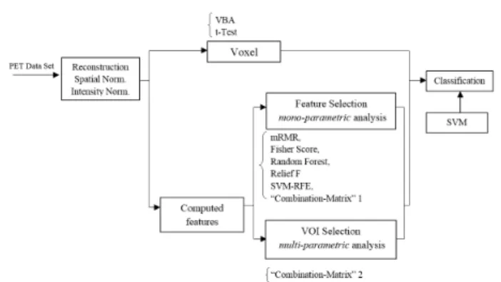
The flowchart of the proposed method is shown in Fig. 1. As for any CAD system, it consists in several important stages:
FIGURE 1. Flowchart of the proposed CAD system.
1. 18F-FDG-PET data acquisition and preprocessing. 2. Computed features
3. Mono-parametric analysis feature selection.
4. Multi-parametric Volume-Of-Interest (VOI) selection and ranking.
5. Classification.
The different stages appearing in this flowchart are detailed in the next sections.
TABLE 1.Demographic details of the dataset.
B. IMAGE DATABASE
FDG PET scans were collected from the ‘‘La Timone’’ University Hospital, in the Nuclear Medicine Department (Marseille, France). The database was built up based on imag-ing studies of subjects that followed the standardized protocol of a hospital-based service. PET scans were performed using an integrated PET/CT camera (Discovery ST, GE Healthcare, Waukesha, USA), with 6.2 mm axial resolution, allowing 47 contiguous transverse sections of the brain of 3.27 mm thickness. 150 MBq of 18FDG were injected intravenously in an awake and resting state, with eyes closed, in a quiet envi-ronment. Image acquisition started 30 min after injection and ended 15 min later. Images were reconstructed using ordered subsets expectation maximization algorithm, with 5 itera-tions and 32 subsets, and corrected for attenuation using CT transmission scan. The local database image enrolled 171 adults 50-90 years of age, including 81 patients with AD and 61 HC and 29 MCI (Mild Cognitive Impairment). Their demographic characteristics are summarized in Table 1. HC were free from neurological/ psychiatric disease and cogni-tive complaints, and had a normal brain MRI. Patients exhib-ited NINCDS-ADRDA [80] clinical criteria for probable AD.
C. IMAGE PREPROCESSING
Images were spatially normalized because of brain volume variation, shape and position from one patient to another. Spatial normalization consisted in applying deformations on volumes so that the whole-brain statistical analysis was per-formed at voxel-level using SPM8 software [43] (Wellcome Department of Cognitive Neurology, University College, London, UK). The data were spatially normalized onto the Montreal Neurological Institute atlas (MNI).This method assumes an affine generic model with 12 parameters [22] and a cost function which presents an extreme value when the image and a template that represents our ‘brain space’ corre-spond to each other. The spatial normalization is achieved by optimizing the quadratic difference between the template and each image. After this spatial normalization, the dimensions of the resulting voxels were 2×2×2 mm and the resulting images of 79×95×68≈5×10⁵voxels size. These images were then smoothed with a Gaussian filter (with different values (0, 4 and 8) of Full Width at Half Maximum (FWHM) to blur individual variations in gyral anatomy and to increase the Signal to Noise Ratio (SNR) [82]. The best FWHM appeared to be 8.
After spatial normalization, intensity normalization was required in order to perform direct images comparison between different subjects. Intensity normalization was nec-essary since global brain activity varies from one subject to another. Different normalization methods were tested [83] to determine the most appropriate one. The retained method consisted in dividing the intensity level of each voxel by the intensity level mean of the gray-matter global brain VOI.
III. FEATURE SELECTION AND VOLUME OF INTEREST RANKING
In this section, we present the main idea of both feature selection and VOI ranking. Brain images are segmented into L VOIs according to AAL of WFU-Pickatlas tool, version 2.4. [84]. Each VOI, Vv,|v{1. . .L} is characterized by a set
of features Pp|p{1. . .K}. The main question that we want
to answer is: how to quantify VOI ability to best distinguish between AD and HC?
Our approach in this work consists in selecting VOIs which best separate between AD and HC classes. Different parameter combinations for each VOI are used to select and rank VOIs according to the ‘‘Area Under Curve’’ (AUC) parameter, defined in the following. The top-ranked VOIs are then introduced into a SVM classifier.
A. NOTATION
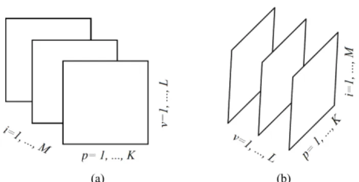
We consider a dataset A RK×L×M. A is a 3-D tensor, where K denotes the number of parameters computed for each VOI amongL VOIs andM is the number of acquired PET images. Let us consider their corresponding metricized version Ai=[A1,A2, . . . ,AM] and Av=[A1,A2, . . . ,AL].
As depicts in Fig. 2, each matrix Aiis of dimensionL×Kand
represents all regional parameters values for cortical VOIs for
FIGURE 2. Frontal (Ai) and lateral (Av) slices of the tensor A that are handled within PET images. (a) Aimatrix of the tensor A. (b) Avmatrix of the tensor A
a selected simplei|i{1. . .M}. Each column of Aiis defined
as volume parameter values computed for all VOIs on the selected simplei. Avis of dimensionM×Kand represents all
simples with parameters values computed on a selected VOI, v|v{1. . .L}.
B. FEATURES DEFINITION
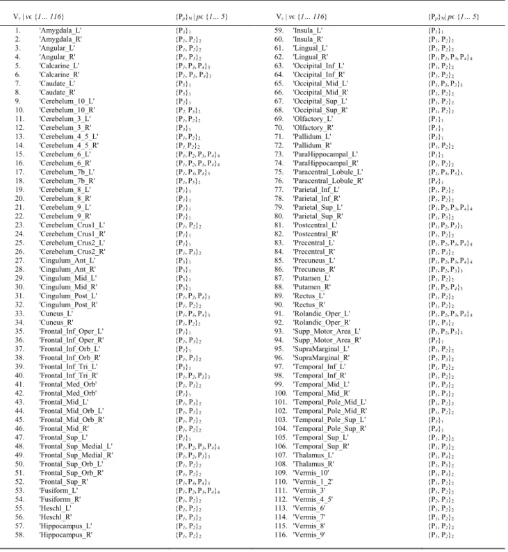
The brain is mapped into 116 cortical VOIs according to AAL of WFU-Pickatlas tool (L = 116). Five parameters (K=5) Pp|p{1. . . 5} are computed for Each VOI, Vv|v{1. . . 116}.
The first order statistics and the entropy were extracted from the histogramh(x) of each VOI :
h(x)= number of voxels in Vvwith gray level x
total number of pixels in the VOI
x∈ {lmin, . . .lmax} (1)
wherexis a gray level value of a voxel belonging to volume Vvandlminandlmaxare the minimum and the maximum gray
level values in Vvrespectively.
P1= Xlmax x=lminxh(x) Mean (2) P2= Xlmax x=lmin(x −P1)2h(x) Variance (3) Pz = Xlmax x=lmin (x−P1)zh(x) (P1)z/2 z{3,4}
Skewness and Kurtosis (4) Ps =
Xlmax
x=lminh(x)log2[h(x)] Entropy (5)
C. AREA UNDER CURVE (AUC) PARAMETER
For each VOI, a set of parameters {Pp|p {1. . . K}} =
{P1, P2, P3, P4, P5} is computed. In the following,
we will use {Pp} instead of {Pp|p {1. . . K}} for
eas-ier readability. HC and AD subjects are plotted in a N feature space, which represents a subset of {Pp},
denoted {Pp}N, N≤K among CNk = N !
(N−K)!K! subsets.
An N-Dimensional sphere (N-D sphere) is created over the group of healthy subjects (HC) (N equals 1 for an interval, 2 for a disk and N is greater than 2 for a sphere). The N-D sphere’s center is the mass center of healthy subjects. At various radii of the N-D sphere, we compute the following parameters:
- nb_HC_in, number of HC subjects inside the N-D sphere,
- nb_AD_in, number of subjects with AD inside the N-D sphere.
- nb_HC_in/nb_HC(1), True Positive Rate (TPR). - nb_AD_in/nb_AD(2), False Positive Rate (FPR).
(1)number of HC subjects in the database(2)number of AD
subjects in the database
The ROC curve is created by plotting the true positives rate (TPR) (i.e. HC subjects well classified) vs. the false positives rate (FPR) (i.e. the AD subjects misclassified) for different radii of the N-D sphere. The AUC is defined as the Area Under ROC Curve (AUC) and is within the range [0, 1]. This AUC quantifies the ability of a given VOI, in a N-D fea-ture space (N≤K) from a subset of K parameters, to separate between groups. This AUC value is all the more near 1 that the subset feature space on which the corresponding VOIs are plotted is able to separate well between AD and HC subjects. Fig. 3 shows the case of ‘Cingulum_Post_Left’ VOI based on three parameters: the mean, the standard deviation and the kurtosis (P1, P2 and P4). The corresponding ROC curve is
shown in Fig. 4.
FIGURE 3. The separation between AD and HC groups relative to the region ’Cingulum_Post_Left with three parameters: the mean, the standard deviation and the kurtosis.
D. ‘‘COMBINATION_MATRIX’’ ANALYSIS
For each VOI, we examine the combination of these parame-ters (noted Pp) with a length varying from 1 toK. Therefore,
we start by the combinations of length 1 ({P1} . . . {PK}), then
those of length 2 ({Pj, Pq}, 1≤j,q≤K,j6=q), and so on until
reaching the combination length of Kparameters. Thereby, we create a ‘‘Combination_Matrix’’ of 2K-1 columns.
For each column, which represents a subset {Pp}N, of N
elements of {Pp}, we compute the AUC (noted αv−N or
αv−{Pp}N) for each VOI, v|v {1. . .L}, according to the
N-D sphere. The ‘‘Combination_Matrix’’ has thenLlines and 2K-1 columns.
1) ‘‘Combination_Matrix’’ 1: mono-parametric analy-sis Based on the ‘‘Combination_Matrix’’, VOIs are ranked according to their higher values of AUC. Each VOI is characterized by its own combina-tion parameters N that gives the highest AUC.
FIGURE 4.ROC curve obtained for region ’Cingulum_Post_Left using three parameters: the mean, the standard-deviation and the kurtosis.
The set of the top ranked VOIs (associated to the higher values of AUC) are selected to be used in AD/HC classification. This is a mono-parametric anal-ysis, in which the selection of VOIs depends only on the combination of the parameters {Pp}N for
each VOI.
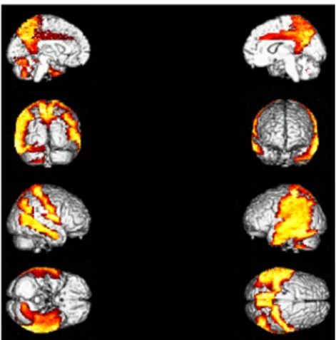
FIGURE 5. The top VOIs (21 VOIs) selected are presented on a 3D brain image
Table 2 gives, for each VOI, the corresponding subset of parameters for which the highest AUC was obtained. The set of best ranked VOIs obtained using AUC approach (21 are given in Table 3 and shown in Fig. 5) are concordant with a recent review of the 18F-FDG PET literature about the positive diagnosis of AD, with VOIs involving the temporo-parietal cortex, includ-ing the precuneus and the adjacent posterior cinclud-ingulate cortex [85].
2) ‘‘Combination_Matrix’’ 2: multi-parametric analysis Multi-parametric analysis for ‘‘Combination_Matrix’’ depends on both the combination of the parameters, (subset of {Pp}), for each VOI, and the combination
TABLE 2. Each VOI Vv|V{1. . .116}is caracterized by its own combination parameters{PP}N.
of the VOIs (subsets of {Vv,|v{1. . . L}}). For
eas-ier readability, we use the expression {Vv} instead
of {Vv | v {1. . . L}}. Depending on the
‘‘Combi-nation_Matrix’’ 1, each VOI is characterized by its own combination of parameters, as it is presented in the Table 2. The procedure begins with the choice of the first two combination VOIs depending on all the possible combinations of VOIs of length 2 ({Vj, Vq},
1≤ j, q≤L, j6= q). Thereafter, a Sequential Forward Selection (SFS) [86] is used where we add one VOI at each step to a VOI list.
So, we start by the combinations of the two VOIs already selected in the previous step, then those of length 3 ({Vj, Vq, Vt}, 1≤j,q,t≤L, j6=q 6=t), and
so on until reaching the combination length of L VOIs. At each step of the iterative procedure, HC and AD
TABLE 3. The list of the top ranked VOIs selected with the best parameters.
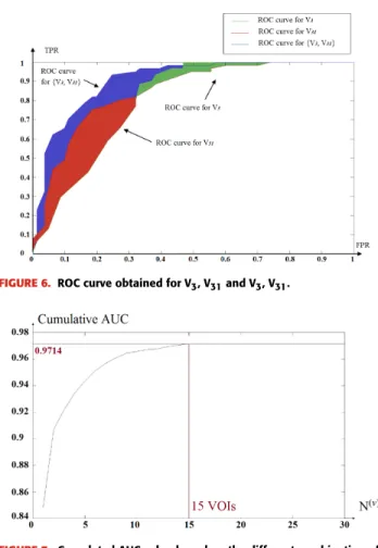
subjects are plotted in a new feature space by combi-nation of parameters for that selection of VOIs. The AUC value based on this combination is named Cumu-lated AUC (CAUC). For easier readability, we use {N(v)} instead of {N(v)| v {1. . . L}}. The VOIs that provide the best CAUC are then added to the final VOIs combination. Our algorithm stops when the same or a lower CAUC is obtained. Then, we select the feature combination with the lowest number of VOIs that achieves the highest CAUC. Fig. 6 shows that the cumulated AUC reaches 0.9071 value when combin-ing V3 and V31, the AUC of which are respectively
0.8012 and 0.8484. The CAUC reached a limit value when more than 15 VOIs were added. This is depicted in Fig. 7.
IV. CLASSIFICATION RESULTS AND DISCUSSION
The result of the proposed algorithm is presented and assessed in this section. However, direct comparison with existing work is hard to achieve due to several factors such as the different datasets, sampling methods, and different features used. We focus on the development and perfor-mance of an algorithm as a whole, while exploring several potential features. In assessing the proposed framework, we provide performance comparison to other feature selection
FIGURE 6. ROC curve obtained for V3, V31and V3, V31.
FIGURE 7. Cumulated AUC value based on the different combination of the VOIs, N(v).
methods using the same local database. The normalized PET database is selected as input data for the CAD tool. PET image of each subject is of 79 × 95 × 68 voxels size, which yields 5×10⁵ voxels. In order to reduce the curse of dimensionality, the 116 VOIs are used first and then the most discriminative VOI among them are then selected. The resulting reduced feature vector obtained from the different PET images is finally taken for classification. In order to validate the effectiveness of the proposed method, we per-formed experiments using a comparison with the state-of-art of Feature Selection methods (FS) including Student’s t-Test analysis [39], Fisher score [86], [87], Support vector Machine feature elimination (SVM-RFE) [88], feature selection with Random Forest [86], [87], [89], minimum Redundancy Max-imum Relevance (mRMR) [64], and ReliefF [63], [90], [91]. The Voxel Based Analysis (VBA), considered as a baseline classification approach is also used for comparison purposes. It consists in inputting to the classifier the whole brain voxels that represent metabolic activity in the gray matter for each subject.
For comparison purposes with feature selection methods but for VBA and Student’s t-Test, a 116x5 matrix, whose lines are VOIs and column are histogram extracted features defined in section III was used. This matrix was input to each FS method in order to obtain the optimal set of features to be input to the SVM classifier.
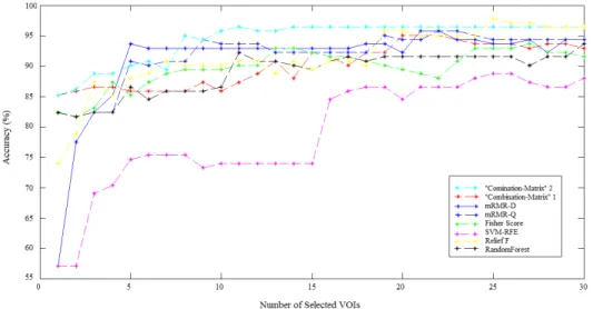
FIGURE 8. Average Accuracy obtained with SVM classifier varying number of features for different VOI selection analyses and applying LOO cross-validation with estimation valueC=10.
FIGURE 9. Average Accuracy obtained with SVM classifier varying number of features for different VOI selection analyses and applying LOO cross-validation with estimation valueC{10−7, 10−6, 10−5. . .102, 103}.
A. CLASSIFICATION RESULTS
Classification was performed using a Support vector machines (SVM) classifier. This classifier map pattern vectors to a high-dimensional feature space where a ‘best’ separating hyperplane (the maximal margin hyperplane) is built. SVM maximize the separation margin by the distance between a hyperplane and the closest data samples. A linear kernel is used our study [86], [87]. Several experiments were carried out to evaluate the ‘‘Combination_Matrix’’ feature selection process and the SVM classifier.
The reduced number of subjects (142 patients) suggests the adaptation of a leave-one-out (LOO) strategy as the most suitable for classification validation. It is a technique that
iteratively holds out a subject for test, while training the clas-sifier with the remaining subjects, so that each subject is left out once. Therefore142training and testing experiments are carried out. Parameter C is used during the training phase and tells how many outliers are taken into account in calculating Support Vectors. For large values ofC, the optimization will choose a smaller-margin hyperplane. Conversely, a very small value ofCwill cause the optimizer to look for a larger-margin separating hyperplane, even if that hyperplane misclassifies more subjects. A good way to estimate relevantC value to be used is to perform it with cross-validation. As a result, the estimation value is fixed to10(C =10) depending upon database. In order to evaluate the developed CAD tool, which
TABLE 4. Voxel selection and VOI selection analyses to discriminate between groups (AD, HC AND MCI).
FIGURE 10. 15 VOIs representation of the‘‘Combination Matrix’’2 on a coronal plane (a), on a transverse plane (b) and on a sagittal plane (c).
depends on the choice ofC, several values ofC are used. The soft-margin constant C of the optimal hyperplane uses a value range from 10−7 to 103, C {10−7, 10−6, 10−5. . . 102, 103}.
Subsequently, performance is also tested using a permu-tation test [92], repeating the classification procedure after randomizing and permuting labels. The p-value is then given by the percentage of runs for which the score obtained is greater than the classification score obtained in the first case. The error of our results were estimated at 0.09% (p-value) for a permutation number equal to1000.
The results achieved using the proposed methods and the SVM are depicted in Fig. 8 and Fig. 9. It illustrates classifica-tion success rate with the different features selecclassifica-tion methods outlined in previous sections. These figures show detailed cross-validation average accuracy results as a function of the number of selected VOIs input to the SVM classifier.
For the whole Feature selection methods, good classification results (above 80% accurate classification rate) are obtained when inputting a low number of VOIs. When the number of VOIs input to the classifier is more than 20, classification results reach a value that remains constant. There is no way to increase classification results by injecting more VOIs. The best accuracy rate obtained by ‘‘Combination_Matrix’’ 1 equals 95.07% (with 19 VOIs), which is higher than the one obtained using VBA which equals 94.36% (see Table 4). The ‘‘Combination_Matrix’’ 2 achieved better results than all the other methods (96.47%) with a lower number of VOIs which are depicted in Fig. 10 (15VOIs).
B. DISCUSSION
A novel approach of feature selection multi-parametric anal-ysis is presented in this paper. The main innovative aspects of this approach rely on the ranking of each anatomical
VOI according to its ability to distinguish between groups of subjects. This method could have been applied to any image data set where a feature selection and ranking is needed. It is also able to give a ranking of a set of VOIs according to their ability to separate groups of subjects. Our study explored two methods: voxel selection and VOI selection analysis applied to 18F-FDG PET data, as well as how to use the parameters in the former approach: mono-parametric or multi-mono-parametric one. The results achieved using the proposed methods are depicted in Table 4. In the case of VBA and t-Test, we talk about voxel approach mono-parametric analysis (voxel is characterized by its intensity). In the case of other classical feature selection methods and ‘‘Combination_Matrix’’ 1, we used a VOI selection mono-parametric analysis. Each VOI was characterized with K parameters. When, we selected the most discriminant VOIs to discriminate between HC and AD patients, each VOI was characterized by one parameter Pp|p {1. . . K} or a set of
parameters computed on it, {Pp}|p{1. . . K}.
In the context of our study, each feature is either a VOI with a combination of parameters computed on it (Combination Matrix 1) or a combination of VOIs, (Com-bination_Matrix 2). After selecting the relevant VOIs, the classification performance was tested by varying the fea-tures vectors dimension and summarized in Tab IV. Our study reduces considerably feature space and computational time. The number of VOIs was reduced to15thanks to ‘‘Combi-nation_Matrix’’ 2 and the computation time was reduced to a few seconds rather than VBA which lasted a day computation time to analyze the whole database.
Even if the main results presented in this paper concern HC versus AD classification, we studied two other possibil-ities. To evaluate the discrimination of MCI (Mild Cognitive Impairment) and AD, we had only 29 patients. Discrimina-tion of MCI from HC is more difficult in comparison to clas-sification of AD from HC (or AD from MCI). We achieved a low performance in discrimination of these groups due to the small number of samples (67.77% with VBA). The best accuracy achieved for discriminating between MCI and AD was 88.18% with ‘‘Combination_Matrix’’ 1, which needs to be evaluated on a larger database. We notice that our approach increases the classification rate for each pair of groups compared to the VBA classification rate, unlike the various classical feature selection methods. ReliefF performed well in the classification between AD and HC, rather than in the case of MCI vs AD and MCI vs HC. The mRMR achieved high accuracy in the case of AD vs HC and MCI vs AD, whereas in the case of MCI vs HC, mRMR features selection achieved lower accuracy values. The obtained results using ‘‘Combi-nation_Matrix’’ 2 for both ‘‘MCI’’ vs ‘‘HC’’ or ‘‘MCI’’ vs ‘‘AD’’ did not achieve good results. This is due to the small number of MCI patients and to the fact that VOIs, in these cases, are more correlated, which did not allow to choose an optimal set of VOIs. Moreover within MCI group we did not distinguish between progressive MCI (pMCI) and stable MCI (sMCI) due to the low number of subjects. Progressive MCI
are subjects that are evolving to an AD state whereas sMCI are subjects that are not going to evolve. The less good results obtained in trying to compare AD to MCI and HC to MCI could be also explained by the fact that AD and pMCI, and also HC and sMCI, are subjects that are hard to distinguish due to the fact that these sub-groups are very close to each other.
VOIs identified and selected in the present work are clas-sically involved in FDG-PET studies of AD, with a bilat-eral metabolic impairment of bilatbilat-eral posterior associative cortices, especially of temporo-parietal regions including the precuneus, and also the posterior cingulate cortex [93].
These results show that the proposed classification results can improve the Computer-Aided Diagnosis of AD on PET images. Therefore, the proposed features selection ‘‘Combi-nation_Matrix’’ is very effective providing a good discrimi-nation between groups and in some cases (due to the small number of samples) comparable results with the various clas-sical feature selection methods.
V. CONCLUSION
In this paper, a novel method for VOIs ranking is developed to better classify brain PET images. This ranking is obtained using ROC curves and quantifies the ability of a VOI to classify HC from AD subjects. A first combination matrix was proposed in order to select relevant features extracted from VOIs then a second combination matrix was able to define best VOIs association for classification purposes.
The Area Under Curve used in this paper could be easily computed for feature selection for any other medical image modality. The evaluation of this parameter was done on a local image database but needs to be evaluated on a larger database.
To go further in the computer aided-diagnosis tasks, other features like texture, gradient computed on VOIs have to be joined to first order statistical parameters in order to enrich information and obtain higher classification results.
REFERENCES
[1] R. Brookmeyer, E. Johnson, K. Ziegler-Graham, and H. M. Arrighi, ‘‘Fore-casting the global burden of Alzheimer’s disease,’’Alzheimer’s Dementia, vol. 3, no. 3, pp. 186–191, Jul. 2007.
[2] Q. Zhouet al., ‘‘An optimal decisional space for the classification of Alzheimer’s disease and mild cognitive impairment,’’IEEE Trans. Biomed. Eng., vol. 61, no. 8, pp. 2245–2253, Aug. 2014.
[3] N. C. Fox and J. M. Schott, ‘‘Imaging cerebral atrophy: Normal ageing to Alzheimer’s disease,’’Lancet, vol. 363, no. 9406, pp. 392–394, Jan. 2004. [4] K. B. Walhovdet al., ‘‘Combining MR imaging, positron-emission tomog-raphy, and CSF biomarkers in the diagnosis and prognosis of Alzheimer disease,’’Amer. J. Neuroradiol., vol. 31, no. 2, pp. 347–354, Feb. 2010. [5] Y. Fan, S. M. Resnick, X. Wu, and C. Davatzikos, ‘‘Structural and
func-tional biomarkers of prodromal Alzheimer’s disease: A high-dimensional pattern classification study,’’Neuroimage, vol. 41, no. 2, pp. 277–285, Jun. 2008.
[6] E. Westman, J.-S. Muehlboeck, and A. Simmons, ‘‘Combining MRI and CSF measures for classification of Alzheimer’s disease and prediction of mild cognitive impairment conversion,’’NeuroImage, vol. 62, no. 1, pp. 229–238, 2012.
[7] P. Vemuriet al., ‘‘MRI and CSF biomarkers in normal, MCI, and AD subjects: Predicting future clinical change,’’Neurology, vol. 73, no. 4, pp. 294–301, Jul. 2009.
[8] K. A. Johnsonet al., ‘‘Preclinical prediction of Alzheimer’s disease using SPECT,’’Neurology, vol. 50, no. 6, pp. 1563–1571, Jun. 1998.
[9] C. Huang, L. Wahlund, T. Dierks, P. Julin, B. Winblad, and V. Jelic, ‘‘Discrimination of Alzheimer’s disease and mild cognitive impairment by equivalent EEG sources: A cross-sectional and longitudinal study,’’Clin. Neurophysiol., vol. 111, no. 11, pp. 1961–1967, Nov. 2000.
[10] G. Henderson et al., ‘‘Development and assessment of methods for detecting dementia using the human electroencephalogram,’’IEEE Trans. Biomed. Eng., vol. 53, no. 8, pp. 1557–1568, Aug. 2006.
[11] D. Zhang, Y. Wang, L. Zhou, H. Yuan, and D. Shen, ‘‘Multimodal classifi-cation of Alzheimer’s disease and mild cognitive impairment,’’ NeuroIm-age, vol. 55, no. 3, pp. 856–867, 2011.
[12] F. Segoviaet al., ‘‘A comparative study of feature extraction methods for the diagnosis of Alzheimer’s disease using the ADNI database,’’ Neuro-computing, vol. 75, no. 1, pp. 64–71, 2012.
[13] B. Dubois et al., ‘‘Research criteria for the diagnosis of Alzheimer’s disease: Revising the NINCDS-ADRDA criteria,’’Lancet. Neurol., vol. 6, no. 8, pp. 734–746, 2007.
[14] G. M. McKhannet al., ‘‘The diagnosis of dementia due to Alzheimer’s dis-ease: Recommendations from the National Institute on Aging-Alzheimer’s association workgroups on diagnostic guidelines for Alzheimer’s disease,’’ Alzheimer’s Dementia, vol. 7, no. 3, pp. 263–269, 2011.
[15] L. Mosconi, V. Berti, L. Glodzik, A. Pupi, S. De Santi, and M. J. de Leon, ‘‘Pre-clinical detection of Alzheimer’s disease using FDG-PET, with or without amyloid imaging,’’J. Alzheimers Disease, vol. 20, no. 3, pp. 843–854, 2010.
[16] D. Perani et al., ‘‘A survey of FDG- and amyloid-PET imaging in dementia and GRADE analysis,’’ BioMed. Res. Int., vol. 2014, Mar. 2014, Art. no. 785039. [Online]. Available: http://dx.doi.org/ 10.1155/2014/785039
[17] X. Wang, B. Nan, J. Zhu, R. Koeppe, and K. Frey, ‘‘Classification of ADNI PET images via regularized 3D functional data analysis,’’Biostat., Epidemiol., vol. 1, no. 1, pp. 3–19, 2017.
[18] J. M. Hoffmanet al., ‘‘FDG PET imaging in patients with pathologically verified dementia,’’J. Nucl. Med., vol. 41, no. 11, pp. 1920–1928, 2000. [19] J. B. Langbaumet al., ‘‘Categorical and correlational analyses of
base-line fluorodeoxyglucose positron emission tomography images from the Alzheimer’s disease neuroimaging initiative (ADNI),’’Neuroimage, vol. 45, no. 4, pp. 1107–1116, 2009.
[20] T. Tuszynskiet al., ‘‘Evaluation of software tools for automated identifica-tion of neuroanatomical structures in quantitativeβ-amyloid PET imaging to diagnose Alzheimer’s disease,’’Eur. J. Nucl. Med. Mole. Imag., vol. 43, no. 6, pp. 1077–1087, Jun. 2016.
[21] S. Mareeswari and G. W. Jiji, ‘‘A survey: Early detection of Alzheimer’s disease using different techniques,’’Int. J. Comput. Sci., Appl., vol. 5, no. 1, pp. 27–37, Feb. 2015.
[22] P. Padillaet al., ‘‘Analysis of SPECT brain images for the diagnosis of Alzheimer’s disease based on NMF for feature extraction,’’Neurosci. Lett., vol. 479, no. 3, pp. 192–196, 2010.
[23] J. Ramírezet al., ‘‘Computer aided diagnosis system for the Alzheimer’s disease based on partial least squares and random forest SPECT image classification,’’Neurosci. Lett., vol. 472, no. 2, pp. 99–103, 2010. [24] M. Fanet al., ‘‘Identification of conversion from mild cognitive
impair-ment to Alzheimer’s disease using multivariate predictors,’’PLoS ONE, vol. 6, no. 7, p. e21896, Jul. 2011.
[25] V. S. Aiswarya and S. Jemimah, ‘‘Diagnosis of Alzheimer’s disease in brain images using pulse coupled neural network,’’Int. J. Innov. Technol. Exploring Eng., vol. 2, no. 6, pp. 2278–3075, May 2013.
[26] I. A. Illán et al., ‘‘18F-FDG PET imaging analysis for computer aided Alzheimer’s diagnosis,’’Inf. Sci., vol. 181, no. 4, pp. 903–916, 2011.
[27] S. Makeig, A. J. Bell, T. P. Jung, and T. J. Sejnowski, ‘‘Independent com-ponent analysis of electroencephalographic data,’’ inAdvances in Neural Information Processing Systems, vol. 8. Cambridge, MA, USA: MIT Press, 1996, pp. 145–151.
[28] F. Segovia, C. Bastin, E. Salmon, J. M. Górriz, J. Ramírez, and C. Phillips, ‘‘Combining PET images and neuropsychological test data for automatic diagnosis of Alzheimer’s disease,’’PLoS ONE, vol. 9, no. 2, p. e8868, Feb. 2014.
[29] M. M. Dessouky, M. A. Elrashidy, and H. M. Abdelkader, ‘‘Select-ing and extract‘‘Select-ing effective features for automated diagnosis of Alzheimer’s disease,’’Int. J. Comput. Appl., vol. 81, no. 4, pp. 17–28, Nov. 2013.
[30] P. Padilla, M. López, J. M. Górriz, J. Ramírez, D. Salas-Gonzalez, and I. Álvarez, ‘‘NMF-SVM based CAD tool applied to functional brain images for the diagnosis of Alzheimer’s disease,’’IEEE Trans. Med. Imag., vol. 31, no. 2, pp. 207–216, Feb. 2012.
[31] F. J. Martínez-Murcia, J. M. Górriz, J. Ramírez, C. G. Puntonet, and I. A. Illán, ‘‘Functional activity maps based on significance measures and independent component analysis,’’Comput. Methods Programs Biomed., vol. 111, no. 1, pp. 255–268, 2013.
[32] P. T. Selvy, V. Palanisamy, and M. S. Radhai, ‘‘A proficient clustering technique to detect CSF level in MRI brain images using PSO algorithm,’’ WSEAS Trans. Comput., vol. 7, no. 7, pp. 298–308, Jul. 2013.
[33] H. Greenspan, A. Ruf, and J. Goldberger, ‘‘Constrained Gaussian mixture model framework for automatic segmentation of MR brain images,’’IEEE Trans. Med. Imag., vol. 25, no. 9, pp. 1233–1245, Sep. 2006.
[34] R. R. Li Perneczky, I. Yakushev, S. Förster, A. Kurz, A. Drzezga, and S. Kramer, ‘‘Gaussian mixture models a nd model selection for [18F] fluorodeoxyglucose positron emission tomography classification in Alzheimer’s disease,’’PLoS ONE, vol. 10, no. 4, p. e0122731, Apr. 2015, doi:10.1371/journal.pone.0122731.
[35] S. J. Hussain, T. S. Savithri, and P. V. S. Devi, ‘‘Segmentation of tissues in brain MRI images using dynamic neuro-fuzzy technique,’’Int. J. Soft Comput. Eng., vol. 1, no. 6, pp. 2231–2307, Jan. 2012.
[36] A. Meena and K. Raja, ‘‘Segmentation of Alzheimer’s disease in PET scan datasets using MATLAB,’’Int. J. Comput. Appl., vol. 57, no. 10, pp. 15–19, Nov. 2012.
[37] A. Abidi, A. B. Tufail, A. M. Siddiqui, and M. S. Younis, ‘‘Automatic classication of initial categories of Alzheimer’s disease from structural MRI phase images: A comparison of PSVM, KNN and ANN methods,’’ Int. J. Biomed. Biol. Eng., vol. 6, no. 12, pp. 713–717, 2012.
[38] M. M. Dessouky, M. A. Elrashidy, E. T. Taha, and H. M. Abdelkader, ‘‘Dimension and complexity study for Alzheimer’s disease feature extrac-tion,’’Int. J. Eng. Comput. Sci., vol. 3, no. 7, pp. 7132–7137, Jul. 2014. [39] X. Long and C. Wyatt, ‘‘An automatic unsupervised classification of MR
images in Alzheimer’s disease,’’ inProc. Comput. Vis. Pattern Recog-nit. (CVPR), Jun. 2010, pp. 2910–2917.
[40] M. T. Hagan and M. B. Menhaj, ‘‘Training feedforward networks with the Marquardt algorithm,’’ IEEE Trans. Neural Netw., vol. 5, no. 6, pp. 989–993, Nov. 1994.
[41] D. E. Rumelhart, G. E. Hinton, and R. J. Williams, ‘‘Learning repre-sentations by back-propagating errors,’’Nature, vol. 323, pp. 533–536, Oct. 1986.
[42] S.-T. Yanget al., ‘‘Discrimination between Alzheimer’s disease and mild cognitive impairment using SOM and PSO-SVM,’’Comput. Math. Meth-ods Med., vol. 2013, Apr. 2013, Art. no. 253670.
[43] K. Friston, J. Ashburner, S. Kiebel, T. Nichols, and W. Penny, Statis-tical Parametric Mapping: The Analysis of Functional Brain Images. Amsterdam, The Netherlands: Academic, 2007.
[44] D. Salas-Gonzálezet al., ‘‘Feature selection using factor analysis for Alzheimer’s diagnosis using F-FDG pet images,’’Med. Phys., vol. 37, no. 11, pp. 6084–6095, 2010.
[45] J. Stoeckel, N. Ayache, G. Malandain, P. M. Koulibaly, K. P. Ebmeier, and J. Darcourt, ‘‘Automatic classification of SPECT images of Alzheimer’s disease patients and control subjects,’’ inMedical Image Computing and Computer-Assisted Intervention—MICCAI (Lecture Notes in Computer Science), vol. 3217. Heidelberg, Germany: Springer, 2004, pp. 654–662. [46] D. Salas-Gonzalezet al., ‘‘Selecting regions of interest in SPECT images
using Wilcoxon test for the diagnosis of Alzheimer’s disease,’’ inProc. 5th Int. Conf. HAIS, San Sebastián, Spain, Jun. 2010, pp. 446–451. [47] W. Zhao, C. Wu, K. Yin, T. Y. Young, and M. D. Ginsberg,
‘‘Pixel-based statistical analysis by a 3D clustering approach: Application to autoradiographic images,’’Comput. Methods Programs Biomed., vol. 83, no. 1, pp. 18–28, 2006.
[48] I. Guyon and A. Elisseeff, ‘‘An introduction to variable and feature selec-tion,’’J. Mach. Learn. Res., vol. 3, pp. 1157–1182, Jan. 2003.
[49] G. Chandrashekar and F. Sahin, ‘‘A survey on feature selection methods,’’ Comput. Elect. Eng., vol. 40, no. 1, pp. 16–28, 2014.
[50] R. Kohavi and G. H. John, ‘‘Wrappers for feature subset selection,’’Artif. Intell., vol. 97, no. 1, pp. 273–324, 1997.
[51] I. Inza, P. Larrañaga, R. Blanco, and A. J. Cerrolaza, ‘‘Filter versus wrapper gene selection approaches in DNA micro array domains,’’Artif. Intell. Med., vol. 31, no. 2, pp. 91–103, 2004.
[52] D. Chyzhyk, A. Savio, and M. Graña, ‘‘Evolutionary ELM wrapper fea-ture selection for Alzheimer’s disease CAD on anatomical brain MRI,’’ Neurocomputing, vol. 128, pp. 73–80, Mar. 2013.
[53] J. Weston, A. Elisseeff, B. Schiölkopf, and M. Tipping, ‘‘Use of the zero norm with linear models and kernel methods,’’J. Mach. Learn. Res., vol. 3, pp. 1439–1461, Mar. 2003.
[54] L. Breiman, J. Friedman, R. Olshen, and C. Stone,Classification and Regression Trees. Monterey, CA, USA: Wadsworth and Brooks, 1984. [55] R. Casanovaet al., ‘‘High dimensional classification of structural MRI
Alzheimer’s disease data based on large scale regularization,’’Front. Neu-roinform., vol. 5, no. 22, pp. 1–9, 2011.
[56] P. M. Morgado, M. Silveira, and J. S. Marques, ‘‘Diagnosis of Alzheimer’s disease using 3D local binary patterns,’’ Comput. Methods Biomech. Biomed. Eng. Imag. Vis., vol. 1, no. 1, pp. 2–12, 2013.
[57] R. Chaves et al., ‘‘SVM-based computer-aided diagnosis of the Alzheimer’s disease using t-test NMSE feature selection with feature correlation weighting,’’Neurosci. Lett., vol. 461, no. 3, pp. 293–297, 2009. [58] E. Bicacro, M. Silveira, and J. S. Marques, ‘‘Alternative feature extraction methods in 3D brain image-based diagnosis of Alzheimer’s disease,’’ inProc. 9th IEEE Int. Conf. Image Process. (ICIP), Sep./Oct. 2012, pp. 1237–1240.
[59] X. He, D. Cai, and P. Niyogi, ‘‘Laplacian score for feature selection,’’ in Proc. Adv. Neural Inf. Process. Syst., 2005, pp. 507–514.
[60] T. M. Mitchell,Machine Learning. New York, NY, USA: McGraw-Hill, 1997.
[61] J. R. Quinlan, ‘‘Induction of decision trees,’’Mach. Learn., vol. 1, no. 1, pp. 81–106, 1986.
[62] J. Yang, Y. Liu, Z. Liu, X. Zhu, and X. Zhang, ‘‘A new feature selec-tion algorithm based on binomial hypothesis testing for spam filtering,’’ Knowl.-Based-Syst., vol. 24, no. 1, pp. 904–914, 2011.
[63] K. Kira and L. A. Rendell, ‘‘The feature selection problem: Traditional methods and a new algorithm,’’ inProc. 10th Nat. Conf. Artif. Intell., 1992, pp. 129–134.
[64] H. Peng, F. Long, and C. Ding, ‘‘Feature selection based on mutual infor-mation criteria of max-dependency, max-relevance, and min-redundancy,’’ IEEE Trans. Pattern Anal. Mach. Intell., vol. 27, no. 8, pp. 1226–1238, Aug. 2005.
[65] F. Fleuret, ‘‘Fast binary feature selection with conditional mutual informa-tion,’’J. Mach. Learn. Res., vol. 5, pp. 1531–1555, Nov. 2004.
[66] B. Guo and M. S. Nixon, ‘‘Gait feature subset selection by mutual infor-mation,’’IEEE Trans. Syst., Man, Cybern. A, Syst., Humans, vol. 39, no. 1, pp. 36–46, Jan. 2009.
[67] P. Mitra, C. A. Murthy, and S. K. Pal, ‘‘Unsupervised feature selection using feature similarity,’’IEEE Trans. Pattern Anal. Mach. Intell., vol. 24, no. 3, pp. 301–312, Mar. 2002.
[68] L. Yu and H. Liu, ‘‘Feature selection for high-dimensional data: A fast correlation-based filter solution,’’ inProc. 20th Int. Conf. Mach. Learn., 2003, pp. 856–863.
[69] L. Yu and H. Liu, ‘‘Efficient feature selection via analysis of relevance and redundancy,’’J. Mach. Learn. Res., vol. 5, pp. 1205–1224, Oct. 2004. [70] A. J. Ferreira and M. A. T. Figueiredo, ‘‘An unsupervised approach to
feature discretization and selection,’’Pattern Recognit., vol. 45, no. 9, pp. 3048–3060, Sep. 2012.
[71] G. Chandrashekar and F. Sahin, ‘‘A survey on feature selection methods,’’ Comput. Elect. Eng., vol. 40, no. 9, pp. 16–28, 2014.
[72] P. M. Morgado and M. Silveira, ‘‘Minimal neighborhood redundancy maximal relevance: Application to the diagnosis of Alzheimer’s disease,’’ Neurocomputing, vol. 155, pp. 230–295, May 2015.
[73] S. Tabakhi and P. Moradi, ‘‘Relevance–redundancy feature selection based on ant colony optimization,’’Pattern Recognit., vol. 48, no. 9, pp. 2798–2811, 2015.
[74] S. Rathore, M. Habes, M. A. Iftikhar, A. Shacklett, and C. Davatzikos, ‘‘A review on neuroimaging-based classification studies and associated feature extraction methods for Alzheimer’s disease and its prodromal stages,’’NeuroImage, vol. 155, pp. 530–548, Jul. 2017.
[75] C. Hinrichs, V. Singh, L. Mukherjee, G. Xu, M. K. Chung, and S. C. Johnson, ‘‘Spatially augmented LPboosting for AD classification with evaluations on the ADNI dataset,’’ Neuroimage, vol. 48, no. 1, pp. 138–149, 2009.
[76] C. Cabral, P. M. Morgado, D. C. Costa, and M. Silveira, ‘‘Predicting conversion from MCI to AD with FDG-PET brain images at different prodromal stages,’’Comput. Biol. Med., vol. 58, pp. 101–109, Mar. 2015. [77] S. F. Eskildsen, P. Coupé, D. García-Lorenzo, V. Fonov, J. C. Pruessner, and D. L. Collins, ‘‘Prediction of Alzheimer’s disease in subjects with mild cognitive impairment from the ADNI cohort using patterns of cortical thinning,’’Neuroimage, vol. 65, pp. 511–521, Jan. 2013.
[78] M. Paganiet al., ‘‘Volume of interest-based [18F] fluorodeoxyglucose PET discriminates MCI converting to Alzheimer’s disease from healthy controls. A European Alzheimer’s disease consortium (EADC) study,’’ Neuroimage Clin., vol. 7, pp. 34–42, Jan. 2015.
[79] K. R. Gray, R. Wolz, R. A. Heckemann, P. Aljabar, A. Hammers, and D. Rueckert, ‘‘Multi-region analysis of longitudinal FDG-PET for the classification of Alzheimer’s disease,’’Neuroimage, vol. 60, no. 1, pp. 221–229, 2012.
[80] G. McKhann, D. Drachman, M. Folstein, R. Katzman, D. Price, and E. M. Stadlan, ‘‘Clinical diagnosis of Alzheimer’s disease report of the NINCDS-ADRDA work group under the auspices of department of health and human services task force on Alzheimer’s disease,’’Neurology, vol. 34, no. 7, pp. 939–944, Jul. 1984.
[81] R. P. Woods, S. T. Grafton, C. J. Holmes, S. R. Cherry, and J. C. Mazziotta, ‘‘Automated image registration: I. General methods and intrasubject, intramodality validation,’’ J. Comput. Assist. Tomograp., vol. 22, no. 1, pp. 139–152, 1998.
[82] J. A. Maldjian, P. J. Laurienti, R. A. Kraft, and J. H. Burdette, ‘‘An automated method for neuroanatomic and cytoarchitectonic atlas-based interrogation of fMRI data sets,’’ NeuroImage, vol. 19, no. 3, pp. 1233–1239, 2003.
[83] I. Garali, M. Adel, S. Takerkart, S. Bourennane, and E. Guedj, ‘‘Brain region of interest selection for 18FDG positrons emission tomography computer-aided image classification,’’ inProc. IEEE Int. Conf. Image Process. Theory Appl. (IPTA), Paris, France, Oct. 2014, pp. 1–5. [84] R. P. Woods, Spatial Transformation Models. San Diego, CA, USA:
Academic, 2000, ch. 29, pp. 465–490.
[85] N. I. Bohnen, D. S. Djang, K. Herholz, Y. Anzai, and S. Minoshima, ‘‘Effectiveness and safety of 18F-FDG PET in the evaluation of dementia: A review of the recent literature,’’J. Nucl. Med., vol. 53, no. 1, pp. 59–71, 2012.
[86] A. R. Webb and K. D. Copsey,Statistical Pattern Recognition, 3rd ed. Chichester, U.K.: Wiley, 2011.
[87] R. O. Duda, P. E. Hart, and D. G. Stork,Pattern Classification, 2nd ed. New York, NY, USA: Wiley, 2001.
[88] I. Guyon, J. Weston, S. Barnhill, and V. Vapnik, ‘‘Gene selection for cancer classification using support vector machines,’’Mach. Learn., vol. 46, nos. 1–3, pp. 389–422, 2002.
[89] A. Liaw and M. Wiener, ‘‘Classification and regression by random forest,’’ R Newslett., vol. 2, no. 3, pp. 18–22, 2002.
[90] M. Robnik-Šikonja and I. Kononenko, ‘‘Theoretical and empirical analysis of ReliefF and RReliefF,’’Mach. Learn. J., vol. 53, nos. 1–2, pp. 23–69, Oct. 2003.
[91] I. Kononenko, ‘‘Estimating attributes: Analysis and extensions of relief,’’ inProc. Eur. Conf. Mach. Learn. (ECML), vol. 784. 1994, pp. 171–182. [92] T. E. Nichols and A. P. Holmes, ‘‘Nonparametric permutation tests for
functional neuroimaging: A primer with examples,’’Hum. Brain Mapping, vol. 15, no. 1, pp. 1–25, 2003.
[93] L. Koricet al., ‘‘Molecular imaging in the diagnosis of Alzheimer’s disease and related disorders,’’ (Paris),Rev. Neurol., vol. 172, no. 12, pp. 725–734, Dec. 2016.