This item was submitted to Loughborough’s Institutional Repository (https://dspace.lboro.ac.uk/) by the author and is made available under the
following Creative Commons Licence conditions.
For the full text of this licence, please go to: http://creativecommons.org/licenses/by-nc-nd/2.5/
Recursive Estimation of Average Vehicle Time Headway
Using Single Inductive Loop Detector Data
Baibing Li
School of Business & Economics Loughborough University
Loughborough LE11 3TU, United Kingdom (Email: [email protected])
Abstract
Vehicle time headway is an important traffic parameter. It affects roadway safety, capacity, and level of service. Single inductive loop detectors are widely deployed in road networks, supplying a wealth of information on the current status of traffic flow. In this paper, we perform Bayesian analysis to online estimate average vehicle time headway using the data collected from a single inductive loop detector. We consider three different scenarios, i.e. light, congested, and disturbed traffic conditions, and have developed a set of unified recursive estimation equations that can be applied to all three scenarios. The computational overhead of updating the estimate is kept to a minimum. The developed recursive method provides an efficient way for the online monitoring of roadway safety and level of service. The method is illustrated using a simulation study and real traffic data.
Keywords: Bayesian analysis; Microscopic flow characteristic; Recursive estimation; Single loop detector; Vehicle time headway
1. Introduction
Single inductive loop detectors are widely deployed in road networks and play a fundamental role in intelligent transportation systems. The measurements provided by a single loop detector include traffic volume and occupancy. Li (2009) investigated the estimation of average vehicle speed using the data from a single loop detector, where the statistical analysis for vehicle speed was based on the measurements on occupancy and was performed conditional on the traffic volume measurements. From the perspective of information extraction, the measurements on traffic volume are not fully utilized. This paper is complementary to the work in Li (2009) and aims to extract the information contained in the measured traffic counts to estimate average vehicle time headway.
Vehicle time headway is one of the most fundamental microscopic characteristics of traffic flow; it affects roadway safety, capacity, and level of service. It is also crucial for the understanding of driver behavior, and plays an important role in car-following theory and microscopic simulation studies (Brackstone et al., 2009; Kim and Zhang, 2011). For instance, the empirical study in Chang and Kao (1991) has shown that lane-changing behavior is closely related to vehicle time headway. Therefore, the information on vehicle time headway can help us have a better understanding about drivers’ behavior in roadways.
Due to the difficulty in data collection, most existing studies on vehicle time headway focus on static analysis. Piao and McDonald (2003) and Marsden et al. (2003) have recently designed a new mobile device for data collection so that differences in driving behavior can be assessed under various traffic conditions. In these studies, car-following data were collected using an instrumented vehicle equipped with a range of sensors allowing the measurement of time gaps between the instrumented vehicle and the following vehicle. However, because of the cost of the device and manpower, this approach cannot be widely
Zhang et al. (2007) considered another approach. They used the data collected from a dual inductive loop detector to analyze vehicle time headway. A dual loop detector can provide information about traffic flow on a vehicle-by-vehicle basis, thus vehicle time headway can be estimated with high accuracy in Zhang et al. (2007). In addition, since the data are recorded automatically, manpower cost is kept to a minimum. However, this approach has a limitation: the devices for data collection, i.e. dual loop detectors, are neither mobile nor widely deployed in road networks so the information on vehicle time headway is available only for the locations where dual loop detectors are deployed. In contrast, the instrumented vehicles used by Piao and McDonald (2003) and Marsden et al. (2003) can be driven to virtually anywhere to collect data so that the differences in drivers’ behavior can be compared. For instance, Marsden et al. (2003) investigated three types of road, i.e. urban motorways, urban arterial roads, and urban streets, in several different sites in the U.K., France, and Germany.
The studies mentioned above are static analysis where the estimate of headway cannot be updated rapidly as a new observation is collected. The obtained results are useful for long-term transport planning or simulation studies but cannot be used for online traffic monitoring in intelligent transport systems.
Compared to dual loop detectors, single inductive loop detectors (ILDs) are cheaper and much more widely installed. In recent years single ILDs have been used to analyze various traffic problems, including the estimation of vehicular speed (Dailey, 1999; Hazelton, 2004; Li, 2009), the detection of accidents (Cheu and Ritchie, 1995; Khan and Ritchie, 1998), and the estimation of travel time (Dailey, 1993; Petty et al., 1998; Liu et al., 2007). Recently, Dailey and Wall (2005) have suggested estimating average vehicle time headway using single loop data. Because single ILDs are deployed in most roadway sections of strategic motorway
networks for data collection, this approach makes online estimation of headway and thus the online monitoring of roadway safety widely feasible.
The approach incorporated in this paper deviates from the conventional methods for headway analysis. It follows the Bayesian approach developed in Li (2009) to estimate the average headway. The aim of this paper is to improve on the estimator developed by Dailey and Wall (2005) by addressing the following issues. First, to accommodate the nature of traffic data that are collected online, we will develop a recursive approach. In contrast to the estimator of Dailey and Wall (2005) that depends only on the single observation collected in the current time interval, the estimate of the average headway parameter in this paper is updated recursively through a Bayesian approach where the current estimate is a weighted average of the previous estimate and the current observation. Since much more information is used in the estimation, it provides potential for improvement on the quality of the estimate. Secondly, as well as a point estimate of average headway, we also provide a measure of uncertainty by calculating the associated Bayesian credible interval and the posterior variance. Finally, we examine vehicle time headway in various traffic conditions, including both light and congested traffic, as well as the traffic disturbed by factors such as traffic signals, car overtaking, and lane changes.
This paper is structured as follows. Section 2 is devoted to problem formulation. In Section 3 we consider the light traffic scenario and investigate recursive estimation of average vehicle time headway. The results are then extended to congested traffic and disturbed traffic conditions in Section 4. A unified algorithm is developed in Section 5. Then in Section 6 numerical analyses are carried out to illustrate the method. Finally, concluding remarks are offered in Section 7. All proofs of theorems are given in Appendix.
2. Problem formulation
2.1. Data from a single ILD
Time headway is the elapsed time between the front of the lead vehicle passing a point on the roadway and the front of the following vehicle passing the same point. Because of the limitations of many commonly used sensors in traffic engineering, most existing studies focus on the average headway in time intervals with a pre-specified duration (see, e.g. Chang and Kao, 1991; Basu and Maitra, 2010). In particular, the measured traffic data from a single ILD are not at the individual vehicle level but rather the relevant information is aggregated over each time interval of fixed duration (say 20 or 30 seconds). Hence in this paper we will focus on the average headway parameter in each time interval during which the traffic data are aggregated.
Now consider a single ILD that measures traffic flow during a time period that is split into a number of successive time intervals, each having a fixed duration of T. During each time interval k, data measured by the single ILD include (see, e.g., Dailey, 1999; Hazelton, 2004; Li, 2009):
traffic volume mk defined to be the number of vehicles entering the front edge of
the ILD in time interval k;
occupancy Ok defined to be the percentage of time that the ILD is occupied in time interval k.
Hence, it is the pair of data {mk,Ok} that are available from the ILD in each time interval k
(k=1,2,…).
Rather than to investigate vehicle time headway using occupancy data Ok as Dailey and
Wall (2005) did, we focus on traffic volume mk. As we shall see later, much attention has been paid to traffic volume and many sophisticated models have been developed for it in traffic engineering. This enables us to investigate time headway under various traffic conditions.
When traffic is light and there are no disturbing factors such as traffic signals and lane changes, the most commonly used model for traffic volume is Poisson distributions:
) ( ~
| Poisson T
mk with 0, (2-1)
where T is the duration of each time interval over which data are aggregated by the single ILD and is the average rate of arrival. Poisson(T) denotes a Poisson distribution with
probability mass function ( ; ) ( ) exp( )/ k!
m
k T T m
m
p k . The reciprocal of the average
rate of arrival , 1/, is the average time headway at the aggregate level, which is the parameter of interest in this paper.
A useful measure to characterize traffic condition in traffic engineering is the ratio of variance to mean volume r. When traffic is light and can be approximately modeled by a Poisson distribution, the ratio is equal to one, r1.
In reality, however, the ratio of variance to mean volume can greatly deviate from unity, indicating that Poisson distributions are no longer a suitable model. In particular, when traffic becomes heavier, freedom to maneuver is diminished and thus the variance of traffic volume is reduced, resulting in a ratio of variance to mean r that is substantially less than 1. In such a traffic condition, binomial distributions are usually more appropriate than Poisson distributions for modeling the traffic volume (Gerlough and Huber, 1975):
)) /( , ( ~ ) , ( | Bin T mk with 0T/()1, (2-2)
where Bin(n,p) denotes a binomial distribution with probability mass function k k n m m k k p p m n p n m p (1 ) ) , ; ( .
The traffic volume mk in equation (2-2) has a mean of T/ with average headway parameter . The variance of the traffic volume mk is equal to (T/){1T/()} which is affected by the diffusion parameter . In particular, the variance approaches zero as
1 ) /(
T , reflecting the fact that for heavily congested traffic the arrival of vehicles per time interval is nearly constant. On the other hand, the statistical model (2-2) collapses to a Poisson distribution (2-1) as T /()0. We also note that the ratio of variance to mean volume r 1T /() is always less than unity for the binomial distribution (2-2). In traffic engineering it has been long known that for congested traffic, binomial distributions give a much better fit to traffic volume than Poisson distributions do.
Next we consider another important scenario where traffic flow is disturbed by factors such as traffic signals, car overtaking, and lane changes. These disturbance factors lead to a larger variability in traffic volume and the ratio of variance to mean becomes substantially greater than 1. Negative binomial distributions are commonly used in this situation (Gerlough and Huber, 1975): ) / , ( ~ ) , ( | Neg bin T mk , (2-3)
where Negbin(a,b) denotes a negative binomial distribution having probability mass
function k m a k k b b b a a m b a m p 1 1 1 1 1 ) , ; ( .
The traffic volume mk in equation (2-3) has a mean of T/ with average headway parameter . The variance of the traffic volume mk is equal to (T/){1T/()} which is affected by the diffusion parameter . In particular, the variance is greatly inflated as
) /(
T becomes large. On the other hand, the statistical model (2-3) collapses to a Poisson
distribution (2-1) as T/()0. In addition, the ratio of variance to mean volume is always greater than unity, r1T/()1, for negative binomial distributions (2-3).
All the three statistical models for traffic volume are frequently applied in the traffic engineering literature although the Poisson distribution is more commonly used (e.g. Hazelton, 2001; Li, 2005). For instance, Basu and Maitra (2010) carried out a survey on a typical working day to collect the 5-min mainstream traffic counts at different junctions. Lan (2001) investigated a traffic flow predictor based on dynamic generalized linear model framework. Both papers used the variance-mean ratio to differentiate the three statistical distributions. In other applications, Nakayama and Takayama (2003), and Kitamura and Nakayama (2007) incorporated binomial distribution to characterize traffic volume, whereas Tian and Wu (2006) assumed a negative binomial distribution in their analysis.
Before concluding this section, we consider an example of real traffic measured by a single ILD on a weekday (Thursday). The single ILD data were downloaded at http://www.its.washington.edu/tdad. The downloaded data included measurements on volume and occupancy during each time interval of duration 20s for twenty-four hours. The ILD is located in the north of Seattle in Interstate-5 with three lanes in both the northbound and southbound directions.
Figure 1 displays the smoothed variance-mean ratio over the time of day in lane 2 and lane 3 for both directions. It can be seen from Figure 1 (upper left and lower left) that except for the early morning period during which the traffic was light and the ratio r was close to unity, traffic was congested in both northbound and southbound lane 2 throughout the day. This was characterized by a low ratio of variance to mean volume, thus suggesting that a binomial distribution model be a better choice than the Poisson.
On the other hand, the third lanes are overtaking lanes. For both the northbound and southbound directions, traffic in lane 3 exhibited a much larger variability during the day (see Figure 1, upper right and lower right) except for the afternoon peak time. Presumably this was the consequence of car overtaking and lane changing. Negative-binomial distributions thus would provide a better fit than Poisson distributions in this situation.
(Figure 1 is about here)
Fig. 1. The smoothed ratio of variance to mean volume over time in northbound lane 2 (upper left), northbound lane 3 (upper right), southbound lane 2 (lower left), and southbound lane 3 (lower right).
3. Recursive estimation of average headway for light traffic
In this section, we consider statistical inference for the average headway parameter under the light traffic condition. Throughout this section it is assumed that there is no disturbing factor so that the traffic volume follows a Poisson distribution (2-1) with probability mass function p(mk;1)(T/)mk exp(T/)/mk!. We shall pool the current observation on
traffic volume and the information obtained in the previous time intervals, and perform Bayesian analysis for the average headway parameter .
3.1. Bayesian inference
We start with the first time interval, k1. It is assumed that during this time interval, there is no prior knowledge about the average headway parameter . Hence, a non-informative prior is used so that the subsequent inference is unaffected by information external to the current data. Throughout this paper, non-informative priors are chosen using
Jeffrey’s principle. For the Poisson distribution p(mk;1), Jeffrey’s principle leads to the following non-informative prior:
2 / 3 2 / 1 ) ( ) ( I p , (3-1)
where I() is the Fisher information for .
Now applying Bayes’ rule to combine prior (3-1) with likelihood (2-1) p(mk;1), we obtain the following posterior distribution of in the first time interval:
) | ( m1 p ( ) ( 1; 1) p m p (T/)(m13/2)exp{T/}.
Hence, the posterior distribution of is an inverse gamma distribution inv(m11/2,T) with a posterior mean equal to 1T/(m11/2) and a posterior variance equal to
) 2 / 3 /( 1 2 1 m
, where inv(,) denotes an inverse gamma distribution having probability
density function g(t){/()}t(1)exp(/t), and () is the gamma function. Let 2
/ 1
1
2 m
. Then the posterior distribution of in time interval k 1 can be rewritten as
) ) 1 ( , (2 2 1 inv .
Now turning to the next time interval k (k=2,3,…), we specify the prior in time interval k
as the posterior obtained in time interval k1: ) ) 1 ( , ( ~invk k k1 , (3-2)
where the prior mean is equal to k1 and the prior variance is equal to /( 2) 2
1
k
k
. The
prior mean represents an estimate of the average headway parameter obtained a priori. The hyper-parameter k is associated with the accuracy of the prior information about . Note that this prior distribution reflects prior knowledge on the average headway parameter for the ‘local’ time interval k only. Throughout the whole time period of interest (e.g., a day), the time headway usually evolves over time and the ‘local’ prior changes accordingly.
Now we apply Bayes’ rule to combine likelihood (2-1) p(mk;1) with prior (3-2). It can be shown by some algebra that the posterior distribution of is
) ) 1 ( , ( ~ |mk inv k mk k mk k , (3-3) where k k k k k 1 (1 )T/m (3-4)
is the posterior mean with weight k (k1)/(kmk 1), and the posterior variance is
P k k k k m V m ) /( 2)ˆ | var( 2 . (3-5)
We use the posterior mean as an estimate of the average headway parameter. Note that the currently observed average headway in time interval k is T/mk which is usually considered as a crude estimate of . From equation (3-4), the current estimate of is a weighted average of the previous estimate k1 and the current crude estimate T/mk.
Now to assess the uncertainty of the estimate, we construct a credible interval for the headway parameter. From the posterior distribution of in (3-3), a 95% credible interval for can be obtained:
(2(k mk 1)k/02.025(2(k mk)),2(k mk 1)k/02.975(2(k mk))), (3-6)
where 2( )
df
is the value for the chi-squared distribution with df degrees of freedom that provides a probability of to the right of the 2(df) value.
Now moving to the next time interval, we treat the posterior distribution (3-3) obtained in time interval k as the prior distribution in time interval k1:
) ) 1 ( , ( ~inv k 1 k 1 k , (3-7)
where the diffusion parameter is updated as k1k mk. Hence, when a new observation
1
k
3.2. Recursive estimation
For real traffic, the average headway parameter evolves slowly over time. To take this into account, we follow Li (2009) and define a forgetting factor so that observations collected at different times are weighted differently, with the latest observations given the largest weights. Specifically, instead of (3-7), the prior distribution is now specified as
) ) 1 ( , ( ~inv k 1 k 1 k ,
where is a forgetting factor lying in the interval (0, 1). This factor does not affect the prior mean of but its prior variance is inflated, reflecting the fact that a priori we are less sure about the current value of due to its evolution. This results in the following algorithm for the recursive estimation of :
Algorithm 1 (the estimation of average vehicle headway).
Given: length of time interval T; forgetting factor ; initial prior parameters: 1 1/2 and 0
0
.
For k=1:K
Step 1. Collect the current measurement on traffic volume mk; Step 2. Calculate weight k (k 1)/(k mk 1);
Step 3. Estimate the average headway parameter by k kk1(1k)T/mk ; Step 4. Calculate the posterior variance VP k2/(k mk 2);
Step 5. Update the diffusion parameter: k1 (k mk); End.
If there is no vehicle passing through the ILD in a time interval k, then according to Bayesian theory the posterior distribution remains the same as the prior distribution. Hence we set k k1 and k1max(1,k).
It is clear that when the forgetting factor becomes larger (smaller), the estimate of average headway becomes smoother (rougher). In particular, when is taken as 0, all information collected previously is discarded and the current estimate is based solely on the current observation T/mk. See Section 5.5 for further discussion on the choice of the forgetting factor.
4. Further extensions
In this section we extend the results obtained in the previous analysis for light traffic to two other scenarios, congested traffic and disturbed traffic.
4.1. Congested traffic
As illustrated in Figure 1, when traffic becomes heavier, traffic volume per time interval is more uniform with smaller variability. To accommodate this nature, the Poisson model will be replaced with binomial distributions (2-2). For simplicity, in this subsection we shall focus on the analysis for the parameter of interest only, i.e. the average headway parameter . The diffusion parameter is assumed to be known from historical data. The estimation of will be investigated in Section 5.
As before, we suppose that we have no prior knowledge about in time interval k 1
and we specify the Jeffrey’s non-informative prior in the following analysis.
2 / 1 2 / 3 )} / /( 1 1 { ) / ( ) ( T T p . (4-1)
Applying Bayes’ rule to combine prior (4-1) with likelihood (2-2) leads to the following posterior distribution of in time interval k 1:
2 / 1 ) 2 / 3 ( 1 1 1 {1 1/( / )} ) / ( ) | ( m T m T m p .
In general, we suppose that the posterior obtained in time interval k1 (k=2,3,…) has the
following form: k k k T T p()(/ )( 1){11/(/ )} .
The posterior obtained in time interval k1 is now specified as the prior in time interval k
which can be rewritten as
k k k k k k k p()(/ 1)( 1){ ( 1)/(/ 1)} (4-2) with a prior mean of k1 kT/{(k 1)}.
Now we apply Bayes’ rule to combine prior distribution (4-2) with the current observation on traffic volume in equation (2-2) to derive the posterior distribution in time interval k. The main result is summarized below:
Theorem 1. Suppose that conditional on , traffic volume mk follows a binomial
distribution (2-2) with a known diffusion parameter . Then for the prior distribution of specified by (4-2), the posterior distribution of cB(/T 1) has an F distribution with degrees of freedom Bk 2(k k mk 1) and Ak 2(k mk) respectively, where
) 1 /( ) ( k k k k k B m m
c is constant. The posterior mean of is given by
k k k k k 1 (1 )T/m (4-3)
2 ) )( 1 )( 1 ( ) | var( mk VP k k mk k k , (4-4)
where VP is defined in equation (3-5). In addition, a 95% credible interval for is
), 1 ) , ( ( ~ (cBk F0.975 Bk Ak ~cBk(F0.025(Bk,Ak)1)),
where c~B cB1(k mk 1)(k )1. F(a,b) is the value for the F distribution with
degrees of freedom a and b that provides a probability of to the right of the F(a,b) value.
Now moving to the next time interval, the posterior distribution obtained in Theorem 1 is treated as the prior distribution in time interval k1. It can be rewritten as
1 1 1 { ( 1)/( / )} ) / ( ) ( ( 1) 1 1 k k k k k k k p (4-5)
with the updated parameters k1 k mk and k1k . The prior distribution in (4-5) has the same functional form as that in equation (4-2). Hence, when a new observation mk1
becomes available, Theorem 1 can be applied again to obtain the posterior distribution in time interval k1 and the estimate of can be updated using equation (4-3). In addition, we note that when k is large, k1k is not small. In this case, equation (4-4) may be
simplified: )} /( ) 1 ( 1 { ) | var( mk VP k mk k . (4-6) 4.2. Disturbed traffic
As shown in Figure 1, when traffic flow is disturbed by factors such as cars overtaking and lane-changing, traffic volume may have larger variability. In this situation, negative binomial distributions provide a better fit. As before, we assume that the diffusion parameter
in equation (2-3) is known. We shall briefly discuss Bayesian analysis for the average
headway parameter below.
First, the Jeffrey’s non-informative prior is specified for time interval k 1.
Lemma 2. For the negative binomial distribution (2-3), the Jeffrey’s non-informative prior is
2 / 1 1 ) / 1 ( ) / ( ) ( T T p . (4-7)
The distribution given in Lemma 2 is a natural conjugate prior of the negative binomial distribution.As demonstrated later in Theorem 2, it is linked to a transformed F distribution.
In general, motivated by Lemma 2, we suppose that the posterior obtained in the time interval k1 has the following form:
) ( 1 ) / 1 ( ) / ( ) ( T k T k k p , which can be rewritten as
) ( 1 ) 1 ( 1) {( 1) ( / )} / ( ) ( k k k k k k k p (4-8)
with a mean of k1kT/{(k 1)}. The distribution in (4-8) is specified as the prior in time interval k. Now we can obtain the posterior in time interval k via Bayes’ rule.
Theorem 2. Suppose that conditional on , traffic volume mk follows a negative binomial
distribution (2-3) with a known diffusion parameter . Then for the prior distribution of specified by (4-8), the posterior distribution of cNB/T has an F distribution with degrees
of freedom Bk 2(k ) and Ak 2(k mk) respectively, where
) /( ) ( k k k NB m
c is constant. The posterior mean of is given by
k k k k k 1 (1 )T/m (4-9)
)} /( ) 1 ( 1 { ) | var( mk VP k mk k . (4-10)
A 95% credible interval for is
(~cNBkF0.975(Bk,Ak),~cNBkF0.025(Bk,Ak)) (4-11)
with ~cNB (k mk 1)/(k mk).
Now we update parameters k1k mk and k1 k so that the posterior
distribution obtained in Theorem 2 can be rewritten as
) ( 1 1 1 1 (1 / ) ) / ( ) ( T k T k k p .
This posterior is treated as the prior distribution in time interval k1. Hence, statistical inference for in time interval k1 can be drawn in a similar manner.
5. A unified algorithm
In this section we will first investigate how to estimate the diffusion parameter and then develop a unified algorithm that can accommodate all three traffic conditions discussed in the previous sections.
5.1. Estimation of the diffusion parameter via the method of moments
In practice, before the foregoing recursive method is applied, the diffusion parameter needs to be estimated from historical data. In this subsection we focus on the method of moments. Suppose that we have collectedsome traffic volumes from the ILD, mk (k=1,…n), under the same traffic condition. The sample mean Eˆ and variance Vˆ can thus be calculated.
We first consider the binomial distribution (2-2). Let E and V denote the theoretical mean and variance of the binomial distribution (2-2) respectively. It is easy to show that
) /( 2 V E E . (5-1)
Hence can be estimated by replacing E and V with their sample counterparts Eˆ and Vˆ .
The estimate of the diffusion parameter in the negative binomial distribution (2-3) can be obtained similarly. Let E and V be the theoretical mean and variance of the distribution (2-3) respectively. Then we can obtain
) /( 2 E V E . (5-2)
Again the method of moments can be used to estimate by replacing E and V with their sample counterparts, Eˆ and Vˆ .
Clearly, when the sample variance Vˆ is sufficiently close to the sample mean Eˆ , the
estimated diffusion parameter ˆ will become very large in both equations (5-1) and (5-2). In this case, a Poisson distribution is a suitable alternative. In fact, as becomes large, the binomial distribution (2-2) and negative binomial distribution (2-3) will approach to the Poisson distribution (2-1) under certain conditions.
In practice, we can split the whole time period of interest (e.g. a day) into a number of relatively small sub-periods during which the traffic flow is approximately stationary. We then estimate the value of for each sub-period. Consequently, throughout the day we can obtain a piecewise function of for the online estimation of the average headway parameter.
In the next subsection, we will investigate a more sophisticated approach to the estimation of the diffusion parameter.
5.2. A Bayesian approach to estimating the diffusion parameter
Next, we take into account of non-stationarity of traffic flow and develop a Bayesian approach to estimating the diffusion parameter . Consider non-stationary traffic flow where average headway evolves over time and is modeled via a random walk:
k k
k
1 with k ~N(0,1/)
where 2 is the precision parameter. Let p(k |k1,) denote the conditional distribution of k and p(1) denote the distribution of the initial headway parameter 1. Suppose that we know little about 1 a priori and p(1) is taken as a uniform distribution over an interval (0,C).
Now consider a sample of n traffic counts, mk (k=1,…,n), collected over n successive time intervals. Let f(mk |k,) denote the binomial distribution (2-2) or negative binomial distribution (2-3). To complete the model specification in Bayesian analysis, we need to specify the priors for and . We use non-informative priors for and in the analysis: the prior g() of is chosen as a gamma distribution Gamma(a1,b1)and the prior g() of
is chosen as a gamma distribution Gamma(a2,b2), where the hyper-parameters ai and bi
(i=1,2) are small.
Applying Bayes’ rule, the posterior distribution is given by
) ( ) ( ) ( ) , | ( ) , | ( ) , , ,..., ( 1 2 1 1 1 f m p p g g f n k k k n k k k n
.The above posterior can be simulated using a numerical approach and the parameter can
be estimated as its posterior mean. For this end, we follow Hazelton (2004) and use the following MCMC algorithm to simulate draws from the above posterior distribution where
) (t k
, (t) and (t) denote the values of k, and in the t-th iteration (t=1,2,…)
respectively:
Algorithm 2 (the estimation of the diffusion parameter).
Step 1. Initialization. t=1. Set k(t) equal to the crude estimate T/mk if mk 0; otherwise ) ( 1 ) ( t k t k
. Set (t) 1 and (t) equal to (5-1) or (5-2), depending on the specified underlying distribution.
Step 2. For k=1:n
(a) Generate a candidate value of average headway in time interval k, (p)
k
, from the
proposal distribution q(), where q() is given by ( 2(),1/ ())
t t
N if k=1; q() is given by N((k(t)1k(t)1)/2,1/(2(t))) if 1<k<n; and q() is given by
) / 1 , ( () () 1 t t n N if k=n.
(b) Define the acceptance probability as
) ) , | ( ) , | ( , 1 min( () () ) ( ) ( 1 t t k k t p k k m f m f r .
Accept k(p) with probability r1. If the candidate is accepted, let k(t1) k(p); otherwise k(t1) k(t).
Step 3. Generate (t1)from the gamma distribution
) ) ( 5 . 0 , 2 / ) 1 ( ( 2 2 ) ( 1 ) ( 1 1
n k t k t k b n a Gamma .Step 4. Generate a candidate value of , (p), from the proposal distribution N((t),2), where is a tuning parameter which can be tuned during the simulation. Define the acceptance probability as ) ) ( ) , | ( ) ( ) , | ( , 1 min( ) ( 1 ) ( ) 1 ( ) ( 1 ) ( ) 1 ( 2 t n k t t k k p n k p t k k g m f g m f r
.Accept (p) with probability r2. If the candidate is accepted, let (t1) (p); otherwise
) ( ) 1 (t t .
Step 5. Update t by t+1 and go to Step 2 until t reaches to a given size.
Overall, the above MCMC algorithm is a mix of Gibbs sampler and Metropolis-Hastings algorithm. In each iteration t, (t1) can be generated straightforwardly. However, the other parameters are drawn using the Metropolis-Hastings algorithm.
5.3. Robustness of the estimate of average headway
Now we extend Algorithm 1 in Section 3.2 to the scenarios of congested traffic and disturbed traffic.
First, we consider the posterior means. Comparing equations (3-4), (4-3), and (4-9) obtained under different traffic conditions, we can see that the three posterior means share a common form of formula:
k k k k k 1 (1 )T/m .
Hence the recursive formula used for the estimation remains unchanged no matter what the traffic condition is and which statistical model is used in the analysis.
However, it should be noted that unlike the ordinary moving average with a constant weight, the developed method uses a traffic-dependent weight to pool information collected over different time intervals since the weight k (k 1)/(k mk 1) depends on the traffic volume per se. For heavier (or lighter) traffic with larger (or smaller) values of traffic volume mk, the weight k for the previous estimate k1 is lower (or higher).
Next we turn to the posterior variances. Similar to Section 3.2, we introduce the forgetting factor and let k1 (k ) with an initial value of 0 0. It is straightforward to obtain k {(1k1)/(1)}. Substituting it into equations (4-4)
average headway under both congested and disturbed traffic conditions can be written in a unified form: )} 1 /( ) 1 )( 1 ]( / ) [( 1 { ) | var( mk VP VE E2 k mk k1 . (5-3)
Note that equation (5-3) also includes the light traffic scenario as its special case: when traffic is light and there is no disturbing factor, in theory we have EV, and thus equation (5-3) collapses to equation (3-5), i.e. var(|mk)VP. Furthermore, when k is large, we have
0
1
k
. Normally this limiting behavior is rapidly achieved. Hence, the posterior variance
(5-3) may be further simplified to be:
)} 1 )( 1 ]( / ) [( 1 { ) | var( 2 k k P k V V E E m m . (5-4)
It can be seen from (5-4) that, although the posterior variances derived under different traffic conditions share the same form of formula (5-4) for computation purposes, the characteristic of uncertainty associated with the estimate differs for different scenarios. In particular, depending on the sign of V E (i.e. positive, negative, or zero), the variability of the posterior estimate is greater than, less than, or equal to the benchmark VP. Hence, compared with that for light traffic, the variability of the posterior estimate is smaller for congested traffic. This is mainly because under the congested traffic condition, freedom to maneuver is diminished and thus the headway between each lead vehicle and the following vehicle becomes more uniform. The decreased variability of traffic volume leads to a smaller posterior variance of the average headway parameter. Likewise, under the condition that traffic is disturbed, the headway between a lead vehicle and the following vehicle varies substantially, resulting in a larger posterior variance of the average headway parameter.
On the basis of the foregoing discussion, Algorithm 1 can be extended for the estimation of the average headway parameter under all three traffic conditions by modifying Step 4:
Step 4. Estimate the posterior variance by VP{1[(VˆEˆ)/Eˆ2](k mk 1)(1)}.
5.4. Forecasting and model validation
It is important to check a built model before it is applied. In practice, however, it is difficult to directly compare the true values of the parameters with the corresponding estimated values since the true values of the parameters of interest are normally unknown. To circumvent this problem, the built models are usually validated by comparing the measurements of the observable variables to the corresponding forecasted values produced by the model. From the perspective of predictivism, it is the accuracy of predictions that is the ultimate test of the built model (Press, 2003).
In this subsection we investigate the issues of forecasting and model validation. For the problem of average headway estimation, let p( |mk) denote the posterior distribution of average headway in time interval k. According to the previous analysis, p(|mk) is given by equation (3-3) or by Theorem 1 or 2, depending on the traffic condition. Let f(mk1|) denote the probability mass function of traffic volume in time interval k+1 that is given by equation (2-1) or (2-2) or (2-3).
The posterior predictive distribution of the traffic volume in the time interval k+1 is defined to be (Press, 2003): p m d m f m m g( k1| k)
( k1| ) ( | k) .Then the one-step-ahead forecast taken as the mean of the posterior predictive distribution is given by mˆk1
xg(x|mk)dx. The following theorem provides the one-step-ahead forecast of the traffic volume.Theorem 3. Suppose that traffic volume mk follows a Poisson distribution (2-1) or a
binomial distribution (2-2) or a negative binomial distribution (2-3). If the initial prior is specified to be non-informative via Jeffrey’s principle, then the one-step-ahead forecast of the traffic volume mk1 can be calculated using a unified formula below:
) / (
ˆk 1 k T k
m , (5-5)
where k (k mk)(k )/[(k mk 1)(k 1)] and by convention we choose
for Poisson distributions so that k collapses to (k mk)/(k mk 1) in this case.
Theorem 3 indicates that the one-step-ahead forecast of the traffic volume mˆk1 obtained in the current time interval k is equal to the duration of the time interval T divided by the current estimate of average headway k and adjusted by a factor of k.
In practice, in order to validate the method developed in this paper, we calculate the one-step-ahead forecast mˆk1 in each time interval k. We then compare mˆk1 to the true traffic
volume mk1 observed in time interval k+1 (k=1,…,n). The overall performance of the developed method is assessed via the root mean squared error (RMSE):
2 / 1 2 2 )} 1 /( ) ˆ ( {
n m m RMSE n k k k . (5-6)This is illustrated in the empirical analysis in Section 6.2.
5.5. Choice of the forgetting factor
In practice, the forgetting factor is usually treated as a tuning parameter so that it is determined experimentally. In this paper, the forgetting factor is chosen in a way such that the overall forecast error measured by RMSE is kept at the minimum level.
Specifically, suppose that we have collected a set of observations mk (k=1,…,n) on
traffic volume during the period of a day that is of research interest. Consider a grid of points from min to max by a step of
~
(0min max 1), for instance, a grid of points between 0.05 to 0.95 by a step of 0.05. For each point taken by , we apply the modified Algorithm 1 to estimate the average headway and to calculate the one-step-ahead forecast of traffic volume using Theorem 3. The forecasted and observed traffic volumes are then compared. The forgetting factor is chosen so that it leads to the minimum RMSE in equation (5-6).
6. Numerical studies
In this section, we first carry out a simulation study and then perform an empirical analysis to examine the performance of the developed method.
6.1. A simulation study
A major advantage of carrying out a simulation study is that the ‘true’ values of the average headway parameter are known a priori so that it is straightforward to assess the performances of different estimation methods in terms of accuracy.
6.1.1. Data generation
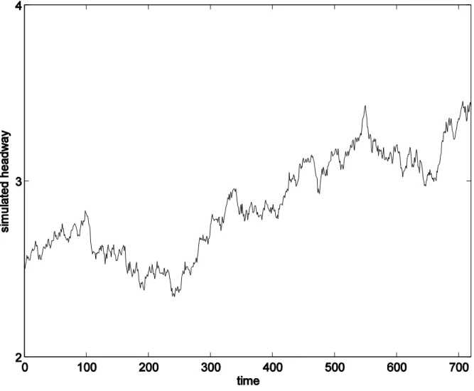
Consider an ILD that measures traffic volume during a number of successive time intervals, each having a duration of T=20s. Traffic flow was simulated in 720 time intervals. To accommodate the nature that vehicle headway evolves slowly over time, the ‘true’ value of the average headway k in time interval k (k=1,…,720) was simulated using a random
walk model having an initial value of 2.5s. The random noise of the random walk followed a normal distribution with a zero mean and a standard deviation of 0.01s. The minimum simulated average headway was set equal to 0.6s in the data generation. The counts mk of
vehicles passing through the ILD were simulated using a negative binomial distribution having a mean of T/k and a diffusion parameter of . The latter parameter was set at different levels in the experiments. Figure 2 displays the simulated values of average headway in one run of the experiments.
(Figure 2 is about here)
Fig. 2. The simulated average headway in one run of the simulation experiments with =10.
6.1.2. Repeated experiments
In the following experiments, the diffusion parameter was set equal to 5, 10, 20 and 50 respectively. In each experiment, the 720 time intervals were split into two sub-periods, one including the first 180 time intervals and the other the remaining 540 intervals. The traffic counts simulated in the first sub-period were treated as the modeling data upon which the diffusion parameter was estimated and the value of the forgetting factor was determined using the method in Section 5. The performance of the developed estimation method was assessed using the data in the second sub-period, where the RMSE between the true values k and the estimated values of average headway ˆk (k=1,…,540) was calculated:
2 / 1 540 1 2 } 540 / ) ˆ ( {
k k k RMSE .In total 100 runs were conducted for each experiment. The developed method was compared with the crude estimate T/mk in terms of average RMSE over the 100 runs, as
displayed in Table 1.
From Table 1, it can be seen that the developed method has a better performance than that of the crude estimation method. This is not surprising: statistically the developed method pools the information collected in the current and previous time intervals via the Bayes’ rule to estimate the average headway, whereas the crude estimation method uses the current observation only.
6.2. A practical example
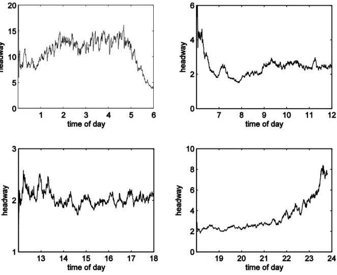
In this subsection we return to the real traffic data discussed in Section 2 and present an empirical analysis for the data. As mentioned before, the collected data includes the counts of vehicles passing through a selected single ILD near Seattle within each 20s time interval during a normal working day (Thursday).
In the following analysis, the whole day of interest was split into four time periods, i.e. midnight to 6 a.m. (period I), 6 a.m. to noon (period II), noon to 6 p.m. (period III), and 6 p.m. to midnight (period IV). For illustration purposes, we consider the traffic in northbound lane 3 only. As shown in Figure 1 (upper right), this includes two important scenarios, disturbed traffic and heavy traffic. The data collected on Thursday is termed testing data hereafter. For the modeling purposes we also downloaded the traffic data one day before (i.e. on Wednesday), termed modeling data hereafter. The diffusion parameter and forgetting factor were determined using the modeling data.
6.2.1. Recursive estimation of average headway
For each time period, we first used the method in Section 5 to determine the forgetting factor based on the modeling data. The modified Algorithm 1 was then applied to the testing data to estimate average headway. The estimated average headway parameter over time is
displayed in Figure 3. It can be seen that during the early morning period, the estimated average headway was between 10s and 15s. In the transition period between 5 a.m. and 7 a.m., it reduced rapidly to about 2s. This level was maintained until about 9 p.m. When the traffic became light in the late evening, it returned to a higher level. These results are in line with those in Zhang et al. (2007) obtained using dual loop detector data.
(Figure 3 is about here)
Fig. 3. The estimated average headway in the periods of midnight to 6 a.m. (upper left), 6 a.m. to noon (upper right), noon to 6 p.m. (lower
left), and 6 p.m. to midnight (lower right).
To evaluate the performance of the developed method, we calculated the RMSEs between the one-step-ahead forecasts of traffic volume mˆ and the observed values k mk using equation (5-6). The accuracy was then compared to the crude estimation method where the forecasted traffic volume was taken as the duration of the time interval T divided by the crude estimate of headway in each time interval.
(Table 2)
It can be seen that the developed method outperformed the crude estimation method: except for the early morning period, the average forecast error of the proposed method is about one vehicle less than that of the crude estimation in each 20s time interval.
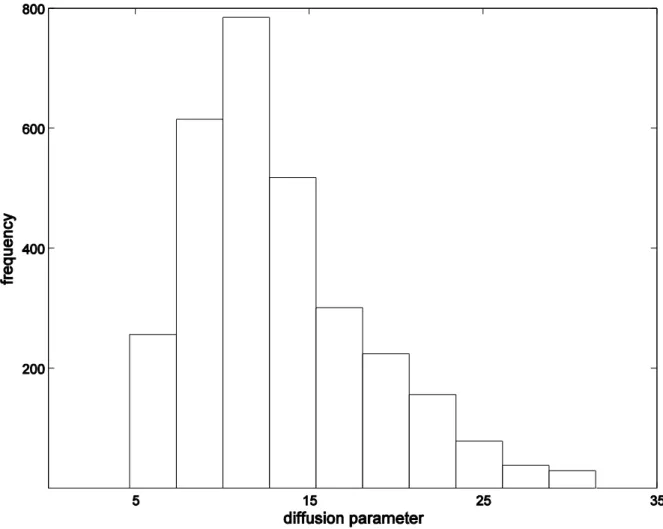
Next, we focus on period I and consider the measure of uncertainty. We first investigate the diffusion parameter using the modeling data in period I. Figure 1 (upper right) suggests that a negative binomial distribution model be suitable for this period.
We carried out a Bayesian analysis outlined in Section 5.2 to estimate the diffusion parameter . For the priors of and , Gamma(a1,b1)and Gamma(a2,b2), we followed
Hazelton (2004) and set the hyper-parameters ai and bi (i=1, 2) equal to 0.001. The upper bound C of p(1) was set equal to 40s.
The posterior distribution was obtained using the MCMC method outlined in Section 5.2. In total 5000 iterations were carried out, where the first 2000 iterations were treated as burnt-in period and thus the correspondburnt-ing results were discarded; the remaburnt-inburnt-ing 3000 draws were retained for the subsequent analysis. The obtained posterior distribution of is displayed in Figure 4. The estimate of using the posterior mean is 15.42 with a posterior standard deviation of 6.02.
(Figure 4 is about here)
Fig. 4. Histogram of 3000 draws from the posterior distribution of parameter using the modeling data in the morning period of
midnight to 6 a.m.
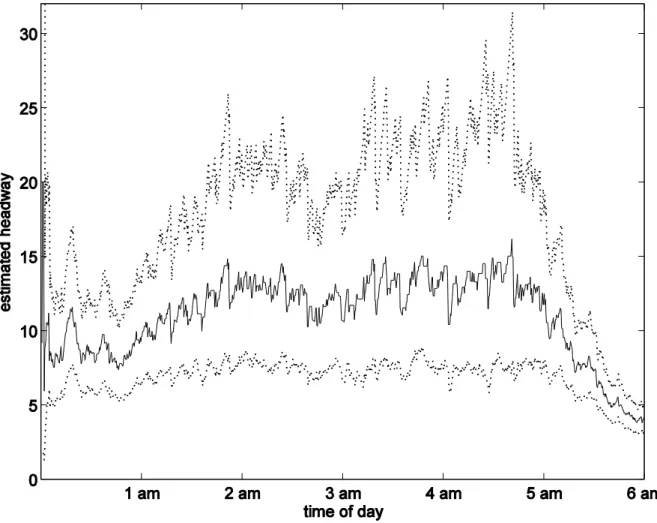
Next we turn to investigate the uncertainty of the average headway estimate. Using the estimated value of from the modeling data, the credible interval for the testing data was constructed, as displayed in Figure 5. It can be seen that although the estimated average headway was mostly around 12s or so before 5 a.m., the envelope of the 95% credible interval was much wider. The upper limit can be as high as 25s or occasionally even over
30s. This is mainly the consequence of the large variability of traffic in this overtaking lane and in this early morning period.
(Figure 5 is about here)
Fig. 5. The estimated average headway in the early morning (real line) and the associated envelope of a nominal 95% credible interval (dotted lines).
7. Concluding remarks
Single inductive loop detectors provide measurements on both traffic volume and occupancy. The research in Li (2009) on vehicular speed estimation used occupancy data and the statistical analysis was performed conditional on traffic volume. This paper is complementary to the work in Li (2009) and aims to extract the information contained in the measurements on traffic volume.
Under three important traffic conditions, i.e. light traffic, heavy traffic, and disturbed traffic, this paper has investigated the estimation of average headway using the data measured from a single ILD. A unified approach has been developed for the recursive estimation of average headway. It shows that the estimates obtained under the three traffic conditions share a common set of recursive equations. Hence, the estimation method is robust in the sense that it does not depend on either the change in traffic condition or the choice for statistical models. The computational overhead of updating the estimate is also kept to a minimum.
Since single ILDs are deployed throughout strategic arterial roadways, this recursive method is applicable in a wide geographical area for online monitoring of roadway safety and the level of service.
The proofs of Lemma 1 and Theorem 1 are given below. Lemma 2 and Theorem 2 can be shown in a similar manner.
Proof of Lemma 1. Let (;mk) denote the probability mass function of the distribution in equation (2-2). Then )} /( 1 log{ ) ( log ) ; ( log mk constmk mk T .
It is easy to verify that
} ) / ( /{ ) / 2 )( ( / / ) ; ( log 2 2 2 2 2 T T m T m mk k k .
Then the Fisher’s information for is equal to
1 3 2 2 ) /( 1 ( } / ) ; ( log { ) ( E m T T I k
and the Jeffrey’s non-informative prior is proportional to
2 / 1
)} (
{I (/T)3/2{11/(/T)}1/2. This completes the proof.
Proof of Theorem 1. Applying Bayes’ rule to combine prior (4-2) with likelihood (2-2) yields the following posterior distribution:
) | ( ) ( ) | ( mk p p mk p (/T)(kmk1){11/(/T)}kkmk .
Let cB(/T1) with constant cB (k mk)/(k k mk 1). It is easy to
verify that random variable follows an F distribution with degrees of freedom ) 1 ( 2 k k k k m
B and Ak 2(k mk) respectively. The posterior mean, posterior
variance, and Bayesian credible interval can be obtained straightforwardly from the F
Proof of Theorem 3. First we note that the one-step-ahead forecast can be calculated using the well-known identity: mˆk1E(mk1|mk)E{E(mk1|mk,)|mk}. It is straightforward to obtain E(mk1|mk,)T/ from equation (2-1) or (2-2) or (2-3), depending on the assumption on the underlying distribution for traffic volume. Hence we have
} | { ˆ 1 1 k k TE m
m . If traffic volume follows Poisson distribution (2-1), the posterior of is
given by (2-3). In this case it is easy to verify that E{1|mk} ( )/( 1)
1 k k k k k m m .
Next we show that Theorem 3 holds when traffic volume follows a binomial distribution (2-2). From Theorem 1, the posterior distribution of cB(/T1) has an F distribution with degrees of freedom Bk 2(k k mk 1) and Ak 2(k mk). We note
} | ) /( { } | { ˆ 1 1 k B B k k TE m E c c m m .
By some algebra the above mathematical expectation can be shown equal to rk(T/k). The proof for the case of the negative binomial distribution is similar.
Acknowledgements
The author would like to thank the two reviewers for their helpful comments on the earlier versions of this paper.
References
Basu, D., Maitra, B., 2010. Evaluation of VMS-based traffic information using multiclass dynamic traffic assignment model: Experience in Kolkata. Journal of Urban Planning and Development 136 (1), 104-113.
Brackstone, M., Waterson, B., McDonald, M., 2009. Determinants of following headway in congested traffic. Transportation Research Part F 12 (2), 131-142.
Chang, G., Kao, Y., 1991. An empirical investigation of macroscopic lane-changing characteristics on uncongested multilane freeways. Transportation Research Part A 25 (6), 375–389.
Cheu, R.L., Ritchie, S.G., 1995. Automated detection of lane blocking freeway incidents using artificial neural networks. Transportation Research Part C 3 (6), 371-388.
Dailey, D. J., 1993. Travel-time estimation using cross-correlation techniques. Transportation Research Part B, 27 (2), 97-107.
Dailey, D. J., 1999. A statistical algorithm for estimating speed from single loop volume and occupancy measurements. Transportation Research Part B 33 (5), 313-322.
Dailey, D. J., Wall, Z. R., 2005. A general simulation model for use with real freeway data to perform congestion prediction - Phase 3. Washington State Transportation Center - TRAC/WSDOT, Final Research Report WA-RD 635.1.
Gerlough, D. L., Huber, M. J., 1975. Traffic Flow Theory: A Monograph. Transportation Research Board, Washington, D.C.
Hazelton, L. M., 2001. Inference for origin-destination matrices: estimation, prediction and reconstruction. Transportation Research Part B 35 (7), 667–676.
Hazelton, M., 2004. Estimating vehicle speed from traffic count and occupancy data. Journal of Data Science 2 (3), 231-244.
Kim, T., Zhang, H. M., 2011. The interrelations of reaction time, driver sensitivity and time headway in congested traffic. The 90th Annual Meeting of the Transportation Research Board, Washington, D.C., January 23-27.
Khan, S. I., Ritchie, S. G., 1998. Statistical and neural classifiers to detect traffic operational problems on urban arterials. Transportation Research Part C 6 (5) 291-314.
Kitamura, R., Nakayama S., 2007. Can travel time information really influence network flow? Implications of the minority game. Transportation Research Record: Journal of the
Transportation Research Board 2010, 12-18.
Lan, C.-J., 2001. A recursive traffic flow predictor based on dynamic generalized linear model framework. IEEE Intelligent Transportation Systems Conference Proceedings – Oakland, USA, August 2001, 25-29.
Li, B., 2005. Bayesian inference for origin-destination matrices of transport networks using the EM algorithm. Technometrics 47 (4), 399-408.
Li, B., 2009. On the recursive estimation of vehicular speed using data from a single inductance loop detector: a Bayesian approach. Transportation Research Part B 43 (4), 391-402.
Liu, H.X., He, X., Recker, W., 2007. Estimation of the time-dependency of values of travel time and its reliability from loop detector data. Transportation Research Part B 41 (4), 448-461.
Marsden, G. R., McDonald, M., Brackstone, M., 2003. A comparative assessment of driving behaviours at three sites. European Journal of Transport and Research 3 (1), 5-20.
Nakayama, S., Takayama, J., 2003. Traffic network equilibrium model for uncertain
demands. The 82th Annual Meeting of the Transportation Research Board, Washington,
D.C., January 12-16.
Petty, K. F., Bickel, P., Ostland, M.; Rice, J., Schoenberg, F., Jiang, J., Ritov, Y., 1998. Accurate estimation of travel times from single-loop detectors. Transportation Research Part A 32 (1), 1-17.
Piao, J., McDonald, M., 2003. Low speed car following behaviour from floating vehicle data. Proc. IEEE Intelligent Vehicles Symposium, Columbus, Ohio, USA, June 2003.
Press, S. J., 2003. Subjective and Objective Bayesian Statistics: Principles, Models and Applications. Wiley, New York.
Tian, Z. Z., Wu, N., 2006. Probabilistic model for signalized intersection capacity with a short right-turn lane. Journal of Transportation Engineering 132 (3), 205-212.
Zhang, G., Wang, Y., Wei, H., Chen, Y., 2007. Examining headway distribution models with urban freeway loop event data. Transportation Research Record 1999, 141-149.
Fig. 1. The smoothed ratio of variance to mean volume over time in northbound lane 2 (upper left), northbound lane 3 (upper right), southbound lane 2 (lower left), and southbound lane 3 (lower right).
Fig. 3. The estimated average headway in the periods of midnight to 6 a.m. (upper left), 6 a.m. to noon (upper right), noon to 6 p.m. (lower left), and 6 p.m. to midnight (lower right).
Fig. 4. Histogram of 3000 draws from the posterior distribution of parameter using the modeling data in the morning period of midnight to 6 a.m.
Fig. 5. The estimated average headway in the early morning (real line) and the associated envelope of a nominal 95% credible interval (dotted lines).
Table 1. Average RMSEs over 100 runs between the ‘true’ and estimated average headways
=5 =10 =20 =50
The developed method 0.40 0.37 0.35 0.35
The crude estimation 3.41 2.89 2.22 1.94
Table 2. RMSEs between the observed traffic volumes and the corresponding one-step-ahead forecasts Period I (midnight – 6:00 a.m.) Period II (6:00 a.m. – 12:00 noon) Period III (12:00 noon – 18:00 p.m.) Period IV (18:00 p.m. – midnight)
The developed method 1.55 3.35 2.90 2.66