Real-Time Distributed Algorithms for Nonconvex Optimal Power Flow
Yuejiang Liu, Jean-Hubert Hours, Giorgos Stathopoulos and Colin N. Jones
Abstract— The optimal power flow (OPF) problem, a funda-mental problem in power systems, is generally nonconvex and computationally challenging for networks with an increasing number of smart devices and real-time control requirements. In this paper, we first investigate a fully distributed approach by means of the augmented Lagrangian and proximal alternating minimization method to solve the nonconvex OPF problem with a convergence guarantee. Given time-critical requirements, we then extend the algorithm to a distributed parametric tracking scheme with practical warm-starting and termination strategies, which aims to provide a closed-loop sub-optimal control policy while taking into account the grid information updated at the time of decision making. The effectiveness of the proposed algorithm for real-time nonconvex OPF problems is demonstrated in numerical simulations.
I. INTRODUCTION
One fundamental problem in the optimization and control of power systems is the optimal power flow (OPF) problem, which seeks to optimize an objective such as generation cost or power loss under certain network constraints such as voltage operation limits and device capacities. The OPF problem is generally nonconvex, and thus NP-hard. Various OPF algorithms have been developed based on convex re-laxations, which are appealing for some particular networks where the relaxation isexact, i.e. the optimal solution of the convex relaxed problem is also a solution of the original OPF problem [17], [18]. However, solving the OPF problem in the case of general networks remains an open and challenging problem.
In addition to non-convexity, the size of the OPF prob-lem poses another challenge to future grid control. Smart devices such as controllable loads and storage elements are increasingly integrated into power grids. On one hand, these devices assist to shave the peak load and compensate for the uncertainties of the electricity demands and renewable energy generations [9], but on the other hand, they inevitably increase the scale and complexity of the OPF problem.
The OPF problem is traditionally solved by a Newton-Raphson method in a centralized manner [14]. However, a distributed method that allows for more agents to simultane-ously participate in the computations is highly desirable for scalability. Some distributed algorithms based on semidefi-nite programming (SDP) or second-order cone programming (SOCP) relaxations for OPF problems have been developed
This work has received support from the European Research Council under the European Unions Seventh Framework Programme (FP/2007-2013)/ ERC Grant Agreement n. 307608 (BuildNet).
Yuejiang Liu,[email protected] Jean-Hubert Hours,[email protected]
Giorgos Stathopoulos,[email protected] Colin N. Jones,[email protected]
for the cases where tight convexification holds [7], [16], [21]. Nevertheless, for the general networks where the convex relaxation is inexact, decomposition needs to take place at the nonconvex level. Recently, [19] and [12] proposed distributed nonconvex OPF algorithms via an alternating minimization method combined with sequential convex approximation or trust region method respectively, but their uses in the real-time scenario are hampered by their reliance on a large number of coordinations between subsystems.
In this work, we aim at solving the nonconvex OPF problem in real-time, as more frequent solutions are re-quested by power networks with increased penetration of renewable energy resources [9]. To achieve this goal, we first tackle the nonconvex OPF problem by a distributed approach with a convergence guarantee. We then further speed it up with practical warm-starting, termination and tuning strategies with the purpose of providing a closed-loop suboptimal control policy, while taking into account the updated grid information at (or close to) the time of decision making. The main contribution of the paper lies in applying the distributed optimization techniques in [2], [11], [13] to the real-time nonconvex OPF problems where the convex relaxation approach [8], [17], [18] fails.
The paper is organized as follows. Section II introduces the formulation of OPF problems. The real-time distributed OPF algorithms are then presented in Section III and tested in Section IV. We finally conclude the paper in Section V.
II. PROBLEMFORMULATION
In this section, we introduce the formulation of the non-convex AC OPF problems considered in the paper.
A. Power Flow Model
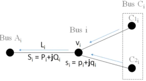
We consider a radial power network T := (N, ε) con-sisting of a set of buses N :={0, ..., n} and a set of lines ε:={1, ..., n}. We index the root node by 0, and denote the rest byN+:=N \{0}. In the network, each busi∈ N+has a set of neighboring buses, including a unique ancestor Ai and a set of children Ci := {C1i, C2i, . . . , Cri, . . . CRi}, and each linei∈εconnects busiand busAi. For each bus
i ∈ N, we denote by Vi the complex voltage, and define
vi := |Vi|
2
. We also denote by si = pi +jqi the power injection at bus i where pi and qi represent the real and reactive power respectively. At the substation bus, the voltage V0 is fixed while the power injection s0 is fully flexible to feed the network. For each line i ∈ ε, let Zi = Ri+jXi denote the complex impedance and Si = Pi+jQi denote the power flow from busito busAi. Also, letIi denote the complex current on the line from busito busAi, and define
Fig. 1. Notations in a radial power network
Li :=|Ii|
2
. The notation of variables is summarized in the table below. The lowercase corresponds to the bus while the uppercase corresponds to the line.
Busi∈ N vi pi qi Linei∈ε(Busi-Ai) Li Pi Qi
Given the network topologyT, the impedanceZ and the substation voltagev0, the power flow in a radial network can be described by the branch flow model [3], [4] as follows:
vAi =vi−2(RiPi+XiQi) +Li(Ri 2 +Xi2) (1a) X Cri∈Ci (PCri−LCriRCri) +pi=Pi (1b) X Cri∈Ci (QCri−LCriXCri) +qi=Qi (1c) Pi2+Qi2=viLi (1d) B. OPF Problem
Two types of constraints commonly exist in grid operation. The first type regards the power injection constraints on the controllable devices at each bus. Suppose that a number of Ki devices such as load, generator and energy storage elements are installed at bus i, the total power injection at this bus is as follows [8]:
pi= Ki X k=1 pi,k, qi= Ki X k=1 qi,k (2)
Letpgeni (t)andqigen(t)denote the active and reactive power injection, respectively, from a generator at timet∈T, which are bounded by:
pgen i ≤p gen i (t)≤p¯ gen i (3a) qgen i ≤q gen i (t)≤q¯ gen i (3b)
For a storage element at busi, letebat
i (t)denote the amount of energy storage andpbat
i (t)denote the discharge rate from the battery to the network at time t ∈ T. The dynamics of the battery are modeled to follow a first-order difference equation with constraints:
ebati (t+ 1) =ebati (t)−pbati (t)∆t (4a) ebati ≤ebati (t)≤e¯bati (4b) pbat i ≤p bat i (t)≤p¯ bat i (4c)
Another operational constraint is on the voltage that is regulated within a range. Suppose that the voltage lower bound and upper bound are defined as vi,v¯i respectively, the voltage at busiis constrained by
vi≤vi≤¯vi (5)
For example, if the allowable voltage deviation is 5% from the nominal, then the voltage at bus i∈ N+ is regulated in a per unit range0.952≤vi≤1.052.
The optimal power flow (OPF) problem typically has an objective function related to the power injections at buses and the currents on the lines, such as minimizing the real power generation or total power losses. Moreover, the objective function is usually an aggregate of the local cost at each agent. In this work, we focus on the following objective function: f(p) = T X t=1 X i∈N {i2(t)(pgeni (t)) 2+ {i1(t)pgeni (t) (6)
where{i2(t)and{i1(t)are the terms associated with gener-ation price at busi at time t. For a network equipped with smart devices such as storage elements or controllable loads, the quadratic cost function tends to shave the peak load and flatten the generation profile, which are favorable for the efficiency of conventional power plants [10].
To summarize, the OPF problem for radial networks is formulated as below:
OPF: min (6)
over v, L, P, Q, p, q s.t. (1),(2),(3),(4),(5)
The equality constraint (1d) is nonconvex. By relaxing this constraint, one can obtain a second-order cone program (SOCP) and gain higher numerical efficiency. However, the solution of the relaxed problem can be infeasible for the grid operation when violating (1d). A detailed analysis regarding the possible inexactness can be found in [15].
III. REAL-TIMEDISTRIBUTEDOPF ALGORITHMS
In this section, we first review a proximal regularized block-coordinate descent method, and then apply it to the nonconvex OPF problem. Subsequently, practical accelera-tion strategies are proposed for the real-time grid operaaccelera-tion. A. Preliminary
The proximal regularized block-coordinate descent method is a powerful framework for solving the minimization problem of a nonconvex function satisfying the Kurdyka-Lojasiewicz property [2]. It tackles the problem of the following structure: min x g(x1, . . . , xp) + p X i=1 hi(xi)
where vector x= (x1, . . . , xp)belongs to the space Rn1×
· · · × Rnp, g is a C1 continuous function with locally Lipschitz continuous gradient, and hi :Rni →
i= 1,2, . . . , p is a proper lower semicontinous function. It is proven in [2] that a bounded sequence {xk1, . . . , xkp}k∈N generated by an inexact block-coordinate descent algorithm converges to a critical point ofg(x1, . . . , xp) +P
p
i=1hi(xi) under the following two assumptions:
Assumption1: (sufficient decrease) For ak
i > 0, the following inequality condition holds:
hi(xki+1) +g(x k+1 1 , . . . , x k+1 i−1, x k+1 i , . . . , x k p) + ak i 2 x k+1 i −x k i 2 ≤hi(xki) +g(x k+1 1 , . . . , x k+1 i−1, x k i, . . . , x k p). (8)
Assumption2: (relative error tolerance) For bk
i >0 and the subgradientvki+1∈∂hi(xki+1), the following inequality condition holds: vki+1+∇xig(x k+1 1 , . . . , x k+1 i , x k i+1, . . . , x k p) ≤bki xki+1−xki . (9) Let us also define the proximal operator and indicator function for the remainder of the paper. Let f : Rn → R∪{+∞}be a proper lower semicontinuous function which is bounded from below, andα >0a positive parameter. The proximal operator off with coefficientαis defined as
proxfα(x) := arg min
y
f(y) +α
2 ky−xk 2
An indicator function of a closed subset Ω of Ris defined as δΩ(x) := 0 ifx∈Ω +∞ ifx /∈Ω B. OPF Decomposition
The OPF problem formulated in Section II has the follow-ing properties that facilitate decomposition:
• The objective function (6) is fully decomposable to each bus in the network.
• The equality constraints (1a - 1c) are linearly coupled between neighboring buses.
• The rest of equality and inequality constraints (1d - 4)
are private at each bus.
Inspired by [20], we first decouple the coupling constraints (1a - 1c) by introducing a set of slack variables xA,i and
xC,i := (xC1,i, xC2,i, . . . , xCr,i, . . .) at bus i as local esti-mates of the coupling variables associated with its neighbors, i.e. an ancestor Ai and a group of childrenCi. Thus, each busimanages a set of local variablesxi:= (xB,i, xA,i, xC,i) as follows: xB,i:=(v (x) i , L (x) i , P (x) i , Q (x) i , p (x) i , q (x) i ) xA,i:=v (x) A,i≡v (x) Ai xCr,i:=(L (x) Cr,i, P (x) Cr,i, Q (x) Cr,i)≡(L (x) Cri, P (x) Cri, Q (x) Cri) where{·}(x) represents local variables.
As the local variablesxA,i, xC,i estimated at busishould be in consensus with the corresponding variables xAi, xCi estimated at the adjacent bus Ai and Ci, a set of slack
variables in charge of communication are defined at the neighborhood around each busi:
zi := (v (z) i , L (z) i , P (z) i , Q (z) i ) where{·}(z) represents consensus variables.
With these additional variables, the OPF problems can be decomposed and reformulated into the following form:
min N X i=1 fi(xi) (11a) s.t. Aixi=bi i∈ N (11b) xTiEixi= 0 i∈ N (11c)
xB,i=zi, xA,i=zAi, xC,i=zCi i∈ N (11d)
xi∈Ωi i∈ N (11e)
where Aixi = bi corresponds to the local linear equality constraints (1a-1c), (2), (4a), xT
iEixi = 0 corresponds to the nonlinear equality constraint (1d), andΩi represents the local inequality bounds (3), (4b-4c), (5) associated withxi.
C. Distributed OPF Algorithm
To tackle the nonconvex OPF problem, we first use the classical augmented Lagrangian method as the outer frame of our algorithms. The augmented Lagrangian associated with the OPF problem (11) is as follows:
Lρ(x, z;µ, γ, λ) =f(x) +µ(Ax−b) +γ(x>Ex) +λ(x−z) +ρ 2kAx−bk 2 +ρ 2 x>Ex 2 +ρ 2kx−zk 2 (12) subject to x ∈ Ω, where Ω := Ω1 × · · · ×Ωn, ρ > 0 is a penalty parameter, x := (x1, . . . , xn) is the group of local variables,z:= (z1, . . . , zn)is the group of consensus variables, µ := (µ1, . . . , µn), γ := (γ1, . . . , γn), λ :=
(λ1, . . . , λn) are Lagrange multipliers associated with the constraints (11b-11d). Specifically, λi := (λB,i, λA,i, λC,i), whereλB,i, λA,i, λC,i correspond to the three different con-sensus constraints associated with (11d).
The standard augmented Lagrangian algorithm solves (11) by the primal-dual sequences:
• Primal update: {xk+1, zk+1}:= arg min x∈Ω,z Lρk(x, z;µk, γk, λk) (13) • Dual update: µk+1:=µk+ρk(Axk+1−b) (14a) γk+1:=γk+ρk(xk+1>Exk+1) (14b) λk+1:=λk+ρk(xk+1−zk+1) (14c) wherekis the iteration indicator.
The dual update is a simple algebraic calculation, which can be split down to each bus for parallel computing. On the contrary, the primal update is a joint minimization of a nonconvex function over two coupling blocks of variables x and z, which is not easy to solve. We will next apply
the proximal block-coordinate descent method to tackle the primal update in a distributed and efficient way.
As described in Section III-B,L(x, z)is fully decompos-able within the varidecompos-able blockxandz:
L(x, z) = N X i=1 Lx,i(xi, z) = N X i=1 Lz,i(x, zi)
where Lx,i and Lz,i are the local augmented Lagrangian functions for the local variablesxi and consensus variables
zi at bus irespectively: Lx,i(xi, z) =fi(xi) +µi(Aixi−bi) + ρ 2kAixi−bik 2 +γi(x>iEixi) + ρ 2 x>iEixi 2 +λi(xB,i−zi) + ρ 2kxB,i−zik 2 +λA,i(xA,i−zAi) + ρ 2kxA,i−zAik 2 + X Cri∈Ci (λCr,i(xCr,i−zCri) + ρ 2kxCr,i−zCrik 2 ) Lz,i(x, zi) =−λi(zi−xB,i) + ρ 2kzi−xB,ik 2 −λCr∗,Ai(zi−xCr∗,Ai) + ρ 2kzi−xCr∗,Aik 2 − X Cri∈Ci (λA,Cri(zi−xA,Cri) + ρ 2kzi−xA,Crik 2 ) +fi(xi) +µi(Aixi−bi) + ρ 2kAixi−bik 2 +γi(x>iEixi) + ρ 2 x>i Eixi 2
where{·}Cr∗,Ai refers to a specific child variable estimated at bus Ai that corresponds to the variable at busi.
It can be noticed that Lx,i is a nonconvex function of
xi andLz,i is a convex function ofzi. Inspired by [6], we tackle the primal update (13) by the following alternating minimization scheme: xmi +1∈arg min xi∈Ωi hxi−xmi ,∇xiLx,i(x m i , z m) i +c m i 2 kxi−x m i k 2 , i∈ N (15) zim+1∈arg min zi Lz,i(xm+1, zi) + dm i 2 kzi−z m i k 2 , i∈ N (16) where m is the iteration indicator, cm
i > 0 and dmi > 0 are the regularization coefficients. In practice, the coefficient dm
i can be taken as a small constant, andcmi can be deter-mined by a backtracking procedure to satisfy the following condition: Lx,i(xmi+1, zm) +α xmi+1−xmi 2 ≤ Lx,i(xmi, zm) +hxmi+1−x m i ,∇xiLx,i(x m i )i+ cm i 2 xmi+1−xmi 2 (17) whereα >0 is a small positive constant.
Proposition 1: Suppose that (17) holds. Then the mini-mization steps (15) and (16) satisfy the inequality (8) and (9).
Proof: The x-update (15) implies hxm+1 i −x m i ,∇xiLxi(x m i )i+ cm i 2 xmi +1−xmi 2 +δΩi(x m+1 i )≤δΩi(x m i ) (18) As the coefficientcm i satisfies (17), we have δΩi(x m+1 i ) +Lx,i(xmi+1) +α xmi+1−xmi 2 ≤δΩi(x m+1 i ) +Lx,i(xmi ) +hxmi+1−x m i,∇xiLx,i(x m i)i+ cm i 2 xmi+1−xmi 2 (19) Substituting (18) into the right side of (19), one obtains
δΩi(x m+1 i ) +Lx,i(xmi+1) +α xmi+1−xmi 2 ≤δΩi(x m i ) +Lx,i(xmi ) (20) By summing up (20) for all the buses, thesufficient decrease assumption (8) is satisfied.
The optimality condition of (15) is
∃vmi +1∈∂δΩi(x m+1 i ), ∇xiLx,i(x m i ) +c m i (x m+1 i −x m i ) +v m+1 i = 0 Then we have vim+1+∇xiLx,i(x m+1 i ) ≤ vim+1+∇xiLx,i(x m i ) + ∇xiLx,i(x m+1 i )− ∇xiLx,i(x m i ) =cmi xmi+1−xmi + ∇xiLx,i(x m+1 i )− ∇xiLx,i(x m i ) ≤(cmi +Li) xmi +1−xmi
whereLi is a Lipschitz constant ofLx,i(xi). Thex-update (15), therefore, satisfies therelative errorassumption (9).
For thez-update, (16) directly implies
Lz,i(zim+1) + dm i 2 z m+1 i −z m i 2 ≤ Lz,i(zmi ) Additionally, the optimality condition of (16) suggests that
∇ziLz,i(z m+1 i ) +d m i (z m+1 i −z m i ) = 0, which implies ∇ziLz,i(z
m+1 i ) ≤ dmi zmi +1−zim .
Thus, thez-update satisfies (8) and (9) as well.
Algorithm 1 Distributed OPF Algorithm
1: Inputs:
grid infomation, inner loop terminiation tolerance, outer loop termination toleranceη
2: Initialize: z, µ, γ, λ, choose ρ >0, β >1 3: repeat 4: repeat 5: xprev, zprev←x, z 6: x←updatexi in parallel (15) 7: z←updatezi in parallel (16) 8: untilk(x−xprev, z−zprev)k ≤/ρ
9: µ, γ, λ← updateµi, γi, λi in parallel (14) 10: ρ←βρ
11: until(Ax−b, x>Ex, x−z) 2≤η
Combining (12-17), our distributed algorithm for the non-convex OPF problem is presented in Algorithm 1. The outer
loop employs the classical augmented Lagrangian method with a growing penalty parameter ρ and a tightening pri-mal update tolerance , while the inner loop follows the proximal regularized alternating minimization framework. As the augmented Lagrangian with a box constraint (12) is a semi-algebraic polynomial function satisfying the Kurdyka-Lojasiewicz (KL) property [5], Algorithm 1 has the following convergence properties.
Theorem1: The sequence {xm, zm} generated by the inner loop of Algorithm 1 converges to a critical point of
Lρ(x, z;µ, γ, λ) +δΩ(x), and it has a finite length.
Proof: The sequence{xm, zm}is constrained by (1-5), and thus Lρ(x, z;µ, γ, λ) +δΩ(x) is bounded from below. Based on Proposition 1, the inner loop of Algorithm 1 is a two-block case of the inexact regularized Gauss-Seidel method, which is proven to converge by Theorem 6.2 in [2].
Theorem2: The sequence{xk, zk, µk, γk, λk}generated by the outer loop of Algorithm 1 converges to a KKT point of Lρ(x, z, µ, γ, λ) +δΩ(x).
Proof: Based on Theorem 1, a proof for the outer loop convergence can be found in [11].
From the computational perspective, Algorithm 1 enables efficient computation at all the agents simultaneously. The x-update (15) minimizes the proximal regularization of the nonconvexLρ(x) linearized at the point xm, and it can be further split into a forward-backward scheme at each busi:
xmi +1=proxδΩi cm i x k i − 1 cm i ∇xiLx,i(x m i , z m)
The backward proximal mapping to the indicator function δΩi(xi) is a projection to a box constraint that has a closed form solution. The z-update (16) can be viewed as a communication step of local variable estimates among the neighborhood around each busi. It minimizes a regularized quadratic function, the solution of which is a system of linear equations and thus can be recovered in closed form as well. As these computations are distributed to each agent, Algorithm 1 is expected to be scalable for large power networks.
D. Real-time Distributed Parametric Tracking
As the OPF problem needs to be solved more and more frequently in a power network with the growing penetration of renewable energy resources, in this section we further investigate practical acceleration strategies with the purpose of providing a highly feasible and suboptimal solution within a limited number of iterations for real-time closed-loop grid operation.
A short-term demand forecast provided by the state-of-art techniques has around 2% - 4% mean absolute percentage error (MAPE) in 24 hours [22], which indicates that the up-dated demand information of a new OPF problem generally does not differ significantly from the demand predicted at the previous time step. This motivates us to initialize the
distributed computation for a new OPF problem from the solution of the previous one:
z0t ←z † t−1,(µ 0 t, γt0, λ0t)←(µ † t−1, γ † t−1λ † t−1) whereztandλtare the consensus variable and multiplier of a new OPF problem solved at timet, and{·}†t−1represents the solution of the previous problem. If the prediction horizon of a multi-stage OPF covers a daily period of time such as 24 hours, we can even warm-start the new problem by the shifted solution of the previous problem to fully take advantage of the solution match. This online warm initialization is expected to provide a good initial guess for solving the new OPF problem, and hence accelerate the online algorithmic performance.
In spite of warm-initialization, Algorithm 1 may still require longer computational time than allowed in the real-time scenario, as the fact that the distributed algorithm based on the first order method generally needs a considerable number of iterations and that the network communication operates at a limited rate much slower than the on-chip exchange. When truncating the iterations of Algorithm 1 is necessary, we would reduce the number of outer loop iterations but maintain the number of inner loop iterations, meanwhile enlarging the penalty parameter ρ in order to provide a highly feasible and suboptimal OPF solution within a limited number of iterations.
Algorithm 2 Distributed OPF Parametric Tracking Scheme
1: Inputs:
grid infomation, allowed number of iterationsM, K new parameters, old solutionzKt−1, µKt−1, γtK−1, λKt−1
2: Initialize: z0t ←ztK−1,(µ0t, γt0, λt0)←(µKt−1, γKt−1λKt−1) chooseρ >0 3: fork= 1,2, . . . , K do 4: form= 1, . . . , M do 5: xm←updatexi in parallel (15) 6: zm←updatezi in parallel (16) 7: end for 8: xk ←xM, zk←zM 9: µk, γk, λk← updateµi, γi, λi in parallel (14) 10: end for
By integrating the initialization and termination strategies into our scheme, a distributed parametric tracking algorithm is presented in Algorithm 2 for the real-time OPF problem. The outer loop of the tracking scheme consists of a fixed number of primal-dual sequences, while the inner loop solves the nonconvex primal update approximately by a fixed number of proximal alternating minimization steps. Provided that the change of OPF parameters, i.e. the load profile and the battery state, over time is relatively slow, it is proven in [13] that the tracking error of Algorithm 2 has the following property:
kwbt+1−w∗t+1k2≤βw(ρ, M)kwbt−wt∗k2 +βs(ρ, M)kst+1−stk2
where βw(ρ, M) =C1(1 +ρC2)(1 + C3 ρ )M − 1 2(3np−1−1) +C 3/ρ βs(ρ, M) =C1(1 +ρC2)C3M − 1 2(3np−1−1) +C3C4/ρ
Here,wbtis the solution at timet,wt∗is the KKT point closest to wbt, st is the parameter of the OPF problem, np ≥ 2 is the number of primal variables,M is number of inner loop iterations, andC1, C2, C3, C4 are constants.
It can be noticed in (21) that in order to ensure the stability of tracking error, βw(ρ, M) and βs(ρ, M) need to be sufficiently small. This motivates us to enlarge the penalty parameterρand the number of inner loop iterations M. By doing so, the contraction of the tracking error is theoretically guaranteed, and thus a series of safety-critical tracking solutions can be provided to the real-time OPF problems.
Remark1: The number of inner loop iterations M that boundsβwandβsto a sufficiently small magnitude needs to grow nonlinearly when the problem dimensionnp increases. However, the choice ofM is restricted by the given compu-tational time and network communication rates in practice.
IV. NUMERICALEXAMPLES
Numerical simulation results are presented in this section to demonstrate that
• Algorithm 1 is capable of solving general nonconvex
OPF problems, for which the convex relaxation ap-proach in [8] fails to provide a feasible solution.
• Algorithm 2 is capable of providing a highly feasible
and suboptimal closed-loop control policy for the OPF problems in real-time grid operation.
Algorithm 1 and 2 are tested on a 9-bus network with 24-hour prediction horizon involving around 4600 variables and 1600 constraints. The network instance is obtained from the test case in [15]. The demand profiles are generated as the product of the static network demand and the normalized hourly demand statistics of European countries [1]. A battery with 0.6 p.u. capacity is artificially inserted into the network, and its stored energy is set to be 0.2 p.u. at 0h every day. A. Offline algorithm convergence
Given plenty of offline computational time, we first solve the nonconvex OPF problem to optimality with Algorithm 1. The initial penalty parameter is set asρ= 1with a growing factorβ = 1.1. The stopping criterion are set as η = 10−4 and = 10−4. Figure 2 shows the feasibility residual and objective value against the outer loop iterations. The feasi-bility error is defined asr=(Ax−b, x>Ex, x−z)
2and
the relative objective difference is defined asf(x)/f(ˆx)−1. Here,xis the OPF solution from Algorithm 1 and xˆ is the solution of the corresponding convex relaxed problem [8]. It can be seen that after 60 outer loop iterations Algorithm 1 converges to a solution that satisfies the feasibility tolerance r = 10−4. In addition, it ends up with an objective value about 2.8% higher than that of a convex relaxed solution,
0 10 20 30 40 50 60 Feasibility Error 10-4 10-3 10-2 10-1 100 Iteration Number 0 10 20 30 40 50 60
Relative Objective Diff-0.04
0 0.04 0.08 0.12
Fig. 2. Feasibility and objective during the iterations of Algorithm 1
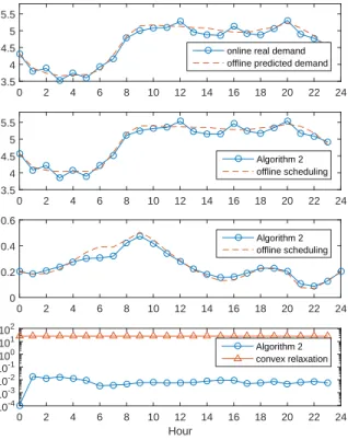
0 2 4 6 8 10 12 14 16 18 20 22 24 Demand (p.u.) 3.5 4 4.5 5 5.5
online real demand offline predicted demand
0 2 4 6 8 10 12 14 16 18 20 22 24 Generation (p.u.)3.5 4 4.5 5 5.5 Algorithm 2 offline scheduling 0 2 4 6 8 10 12 14 16 18 20 22 24
Battery Energy (p.u.) 0
0.2 0.4 0.6 Algorithm 2 offline scheduling Hour 0 2 4 6 8 10 12 14 16 18 20 22 24 Feasiblity Error 10-4 10-3 10-2 10-1 100 101 102 Algorithm 2 convex relaxation
Fig. 3. Closed-loop grid operation controlled by Algorithm 2
which suffers large feasibility error r = 26.6 due to its violation of the nonconvex equality constraint (1d).
B. Online closed loop operation
For the online grid operation, we assume a 24h demand forecast service updated on an hourly basis, and solve the OPF problems with the updated grid information at each hour repeatedly. The demand forecast error is artificially created by shifting the demand periodically with a random perturbation up to 4%. Figure 3 shows the performance of Algorithm 2 with 10 outer loop iterations, maximum 500 inner loop iterations and a penalty parameter ρ= 1. It can be seen that under the closed loop control of Algorithm 2 the
operations of the generators and batteries are different from the day-ahead scheduling and adapt to the online demand changes. We can also observe that the feasibility errors of the truncated real-time solutions remain at a relatively low level, significantly better than the solution of the convex relaxation approach. This demonstrates the potential of Algorithm 2 in providing a highly feasible and sub-optimal control policy for the real-time grid operation.
V. CONCLUSION
Distributed algorithms based on the augmented La-grangian method and proximal alternating minimization tech-niques were proposed to address the nonconvex OPF problem whenever the convex relaxation fails to be exact, either in a network with mesh topology or in a radial network where the convexified OPF solution violates the noncon-vex constraint. Compared with centralized approaches, our distributed algorithms split the computations to each agent, hence are more scalable and privacy-sensitive. Furthermore, the proposed real-time OPF tracking scheme can potentially provide a highly feasible solution within a limited number of agent coordinations when feasibility prioritizes, meanwhile sub-optimally controlling power flow and smart devices for closed-loop grid operation in real-time.
REFERENCES
[1] European network of transmission system operators for electricity, 2014. www.entsoe.eu.
[2] H. Attouch, J. Bolte, and B. F. Svaiter. Convergence of descent methods for semi-algebraic and tame problems: proximal algorithms, forwardbackward splitting, and regularized GaussSeidel methods. Mathematical Programming, 137(1-2):91–129, August 2011. [3] M.E. Baran and F.F. Wu. Optimal capacitor placement on radial
distribution systems.IEEE Transactions on Power Delivery, 4(1):725– 734, January 1989.
[4] M.E. Baran and F.F. Wu. Optimal sizing of capacitors placed on a radial distribution system. IEEE Transactions on Power Delivery, 4(1):735–743, January 1989.
[5] J. Bolte, A. Daniilidis, and A. Lewis. The ojasiewicz Inequality for Nonsmooth Subanalytic Functions with Applications to Subgradient Dynamical Systems.SIAM Journal on Optimization, 17(4):1205–1223, January 2007.
[6] J. Bolte, S. Sabach, and S. Teboulle. Proximal alternating linearized minimization for nonconvex and nonsmooth problems. Mathematical Programming, 146(1-2):459–494, July 2013.
[7] E. Dall’Anese, Hao Zhu, and G.B. Giannakis. Distributed Optimal Power Flow for Smart Microgrids.IEEE Transactions on Smart Grid, 4(3):1464–1475, September 2013.
[8] L. Gan, N. Li, U. Topcu, and S.H. Low. Exact Convex Relaxation of Optimal Power Flow in Radial Networks. IEEE Transactions on Automatic Control, 60(1):72–87, January 2015.
[9] L. Gan, A. Wierman, U. Topcu, N. Chen, and S. H. Low. Real-time Deferrable Load Control: Handling the Uncertainties of Renewable Generation. InProceedings of the Fourth International Conference on Future Energy Systems, e-Energy ’13, pages 113–124, New York, NY, USA, 2013. ACM.
[10] D. Gayme and U. Topcu. Optimal power flow with large-scale storage integration. IEEE Transactions on Power Systems, 28(2):709–717, May 2013.
[11] J.-H. Hours and C.N. Jones. An augmented Lagrangian coordination-decomposition algorithm for solving distributed non-convex programs. InAmerican Control Conference (ACC), 2014, pages 4312–4317, June 2014.
[12] J.-H. Hours and C.N. Jones. An Alternating Trust Region Algorithm for Distributed Linearly Constrained Nonlinear Programs, Application to the AC Optimal Power Flow. arXiv:1502.03777 [math], February 2015. arXiv: 1502.03777.
[13] J.-H. Hours and C.N. Jones. A Parametric Non-Convex Decomposition Algorithm for Real-Time and Distributed NMPC.IEEE Transactions on Automatic Control, PP(99):1–1, 2015.
[14] M.R. Irving and M.J.H. Sterling. Efficient Newton-Raphson algo-rithm for load-flow calculation in transmission and distribution net-works. Generation, Transmission and Distribution, IEE Proceedings C, 134(5):325–330, September 1987.
[15] B. Kocuk, S.S. Dey, and X.A. Sun. Inexactness of SDP Relaxation and Valid Inequalities for Optimal Power Flow. IEEE Transactions on Power Systems, PP(99):1–10, 2015.
[16] A.Y.S. Lam, Baosen Zhang, and D.N. Tse. Distributed algorithms for optimal power flow problem. In2012 IEEE 51st Annual Conference on Decision and Control (CDC), pages 430–437, December 2012. [17] S.H. Low. Convex Relaxation of Optimal Power Flow - Part I:
Formulations and Equivalence. IEEE Transactions on Control of Network Systems, 1(1):15–27, March 2014.
[18] S.H. Low. Convex Relaxation of Optimal Power Flow - Part II: Exactness. IEEE Transactions on Control of Network Systems, 1(2):177–189, June 2014.
[19] S. Magnsson, P. C. Weeraddana, and C. Fischione. A Distributed Approach for the Optimal Power Flow Problem Based on ADMM and Sequential Convex Approximations.arXiv:1401.4621 [math], January 2014. arXiv: 1401.4621.
[20] Q. Peng and S. H. Low. Distributed Optimal Power Flow Algorithm for Balanced Radial Distribution Networks.arXiv:1404.0700 [math], April 2014. arXiv: 1404.0700.
[21] P. Sulc, S. Backhaus, and M. Chertkov. Optimal Distributed Control of Reactive Power Via the Alternating Direction Method of Multipliers. IEEE Transactions on Energy Conversion, 29(4):968–977, December 2014.
[22] J. W. Taylor. Triple seasonal methods for short-term electricity demand forecasting. European Journal of Operational Research, 204(1):139– 152, July 2010.