University of Pennsylvania
ScholarlyCommons
Publicly Accessible Penn Dissertations
1-1-2015
Automated Analysis in Generic Groups
Edvard Olav Valter Fagerholm
University of Pennsylvania, [email protected]
Follow this and additional works at:http://repository.upenn.edu/edissertations Part of theComputer Sciences Commons, and theMathematics Commons
This paper is posted at ScholarlyCommons.http://repository.upenn.edu/edissertations/1053 For more information, please [email protected].
Recommended Citation
Automated Analysis in Generic Groups
Abstract
This thesis studies automated methods for analyzing hardness assumptions in generic group models, following ideas of symbolic cryptography. We define a broad class of generic and symbolic group models for different settings---symmetric or asymmetric (leveled) k-linear groups - and prove ''computational soundness'' theorems for the symbolic models. Based on this result, we formulate a master theorem that relates the hardness of an assumption to solving problems in polynomial algebra. We systematically analyze these problems identifying different classes of assumptions and obtain decidability and undecidability results. Then, we develop automated procedures for verifying the conditions of our master theorems, and thus the validity of hardness assumptions in generic group models. The concrete outcome is an automated tool, the Generic Group Analyzer, which takes as input the statement of an assumption, and outputs either a proof of its generic hardness or shows an algebraic attack against the assumption.
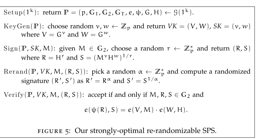
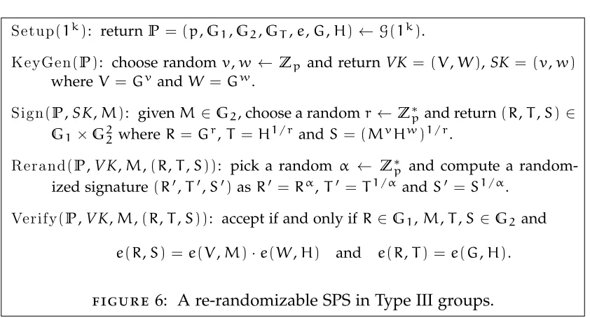
Structure-preserving signatures are signature schemes defined over bilinear groups in which messages, public keys and signatures are group elements, and the verification algorithm consists of evaluating ''pairing-product equations''. Recent work on structure-preserving signatures studies optimality of these schemes in terms of the number of group elements needed in the verification key and the signature, and the number of pairing-product equations in the verification algorithm. While the size of keys and signatures is crucial for many applications, another aspect of performance is the time it takes to verify a signature. The most expensive operation during verification is the computation of pairings. However, the concrete number of pairings is not captured by the number of pairing-product equations considered in earlier work.
We consider the question of what is the minimal number of pairing computations needed to verify structure-preserving signatures. We build an automated tool to search for structure-structure-preserving signatures matching a template. Through exhaustive search we conjecture lower bounds for the number of pairings required in the Type~II setting and prove our conjecture to be true. Finally, our tool exhibits examples of structure-preserving signatures matching the lower bounds, which proves tightness of our bounds, as well as improves on previously known structure-preserving signature schemes.
Degree Type
Dissertation
Degree Name
Doctor of Philosophy (PhD)
Graduate Group
Mathematics
First Advisor
Andre Scedrov
Keywords
Subject Categories
A U T O M AT E D A N A LY S I S I N
G E N E R I C G R O U P S
Edvard Fagerholm
A D I S S E R TAT I O N
in
Mathematics
Presented to the Faculties of
The University of Pennsylvania
in Partial Fulfillment of the Requirements for
the Degree of
Doctor of Philosophy
2015
Andre Scedrov, Professor of Mathematics
Supervisor of Dissertation
David Harbater, Christopher H. Browne Distinguished Professor
Professor of Mathematics
Graduate Group Chairperson
Dissertation Committee:
Andre Scedrov, Professor of Mathematics Gilles Barthe, Professor
A U T O M AT E D A N A LY S I S I N G E N E R I C G R O U P S
© 2015
A C K N O W L E D G E M E N T S
It feels somewhat strange that the period of my life called “doctoral studies” is coming to and end. In six years, surprisingly many things happen. I’ve had the chance to explore Philadelphia, which after some initial shock due to apartment choices, ended up being a wonderful place to live as well as a place that one could start calling home. Friends in the Ph.D. program have come and gone and are now dispersed around the globe. My daughter Ada was born and she has given me more joy than I ever could have imagined. Finally, through all this time, my wife Kaisa has always been there to support me even when it seemed like there was no light at the end of the tunnel.
Finishing a Ph.D., however, is something that one never could have done with-out help from many people. First and foremost, I must thank my advisor Andre Scedrov who has provided me with more flexibility than one could hope to ask for. My wife was able to accept a job offer with the UN in Rome, Italy, after our daughter was born, because Andre suggested that I visit the IMDEA Software Institute in Madrid. A big thank you also goes to my coauthors, especially Gilles Barthe at IMDEA who agreed to host me as well as Dario Fiore and Benedikt Schmidt who both have taught me a great deal and were always available for questions and discussions when needed.
Finally, I would never have survived without the support of other students in the program. In no particular order, I would especially like to thank Taisong Jing, Jonathan Kariv, Tyler Kelly and David Lonoff. Taisong was instrumental in in-troducing me to authentic Chinese food, John would never miss an opportunity to discuss anything related to powerlifting or to comment “do you mean kilos?” when you had made a record at the gym and told him what you lifted (which obviously was in pounds), Tyler is Tyler and, finally, David and I had many inter-esting discussions during the first two years of the Ph.D. program.
None of this would of course have been possible without funding. The work on this thesis was supported in part by ONR grant N00014-12-1-0914 with ad-ditional support from the AFOSR MURI “Science of Cyber Security: Modeling,
A B S T R A C T
A U T O M AT E D A N A LY S I S I N G E N E R I C G R O U P S
Edvard Fagerholm
Andre Scedrov
This thesis studies automated methods for analyzing hardness assumptions
in generic group models, following ideas of symbolic cryptography. We
de-fine a broad class of generic and symbolic group models for different settings—
symmetric or asymmetric (leveled) k-linear groups—and prove “computational
soundness” theorems for the symbolic models. Based on this result, we formulate a master theorem that relates the hardness of an assumption to solving problems in polynomial algebra. We systematically analyze these problems identifying dif-ferent classes of assumptions and obtain decidability and undecidability results. Then, we develop automated procedures for verifying the conditions of our mas-ter theorems, and thus the validity of hardness assumptions in generic group models. The concrete outcome is an automated tool, the Generic Group Analyzer, which takes as input the statement of an assumption, and outputs either a proof of its generic hardness or shows an algebraic attack against the assumption.
C O N T E N T S
a c k n o w l e d g e m e n t s iv
a b s t r a c t v
p r e f a c e ix
1 a p r i m e r o n s o m e t o p i c s i n c r y p t o g r a p h y 1
1.1 Pairings and Multilinear Maps 1
1.2 Signature Schemes 5
2 t h e g e n e r i c g r o u p m o d e l 8
2.1 The Definitions of Shoup and Maurer 8
2.2 Group Settings 11
2.3 Extending Maurer’s Definition 14
2.4 The Schwarz-Zippel Lemma 16
2.5 A Few Proof Examples 18
2.6 Types of Cryptographic Assumptions 24
3 p r o o f au t o m at i o n i n t h e g e n e r i c g r o u p m o d e l 27
3.1 The Symbolic Group Model 28
3.2 Our Master Theorem 30
3.3 Non-Parametric Assumptions 33
3.4 Parametric Assumptions 36
3.5 Interactive Assumptions 43
3.5.1 Automated Analysis 50
3.6 Composite-Order Groups 52
3.6.1 Generic and symbolic model for composite-order bilinear
groups 53
3.6.2 Master Theorem 56
3.6.3 Non-parametric and Non-interactive Assumptions 57
3.7 Rational Input Distributions 57
3.8 Examples 59
4 s t r u c t u r e-p r e s e r v i n g s i g nat u r e s c h e m e s 63
4.2 Known Lower Bounds of Type II SPS 65
4.3 Lower Bounds on the Number of Pairings 66
4.3.1 Main result 66
4.3.2 Gaps in Bounds Between EUF-RMA and EUF-CMA
-Security 68
4.3.3 Proof of Lemma52 69
4.4 SPS Schemes With Verification Key (V,W)∈G1×G2 73
4.5 Synthesis of SPS 82
4.5.1 Generation of Schemes 82
4.5.2 Proof and Attack Search 84
4.5.3 Synthesized Schemes 84
4.5.4 New SPS Schemes 85
5 s u m m a r y o f c o n t r i b u t i o n s 96
5.1 Generalizing the Generic Group Model 96
5.2 Master Theorems for the Extended GGM 96
5.3 Automated Analysis in the Extended GGM 97
5.4 Synthesis of SPS and New SPS Schemes 97
5.5 New Lower Bounds for SPS 98
P R E FA C E
The motivation behind this thesis is to increase trust in security proofs in cryptog-raphy. In the last decade or so a development within cryptography has been to push the boundary on new features provided by cryptographic primitives [BF03, BBG05a, HL02, GPSW06, LOS+10, Gen09], but at the same time relax-ing the standard for security assumptions. While the security of cryptographic primitives used to rely on well-known and long-studied problems, such as the hardness of factoring and the discrete logarithm assumptions, cryptographers started inventing new assumptions while justifying the security of their assump-tions in restricted computational models. The generic group model studied and extended in this thesis is one particularly common example while inventing new assumptions is especially prevalent within the field of pairing-based cryptogra-phy [KM10]. This has lead to a plethora of new security assumptions.
Worrying about this state-of-affairs is not new. In 2005, Halevi wrote a paper
[Hal05], where he noted that “we generate more proofs than we carefully
ver-ify (and as a consequence some of our published proofs are incorrect)”. Indeed, a paper was recently accepted to one of the flagship conferences in cryptogra-phy, ASIACRYPT, which had a faulty generic group proof [HS14, Fuc14, Pan14]. Halevi also noted that some of the reasons for this problem are social: “we mostly publish in conferences rather than journals”. As a solution Halevi proposed writ-ing a tool that could be used to verify the “mundane” parts of cryptographic proofs. Halevi’s paper eventually led to Barthe et. al developing the CertiCrypt [BGZB09] and later the EasyCrypt [BGHZ11] proof assistants for writing mechan-ically verified cryptographic proofs. However, tools like EasyCrypt still have a fairly steep learning curve as well as requiring significant effort from the user compared to writing manual proofs. Unfortunately, this is currently a price to pay for mechanically verified proofs, which is shared by most proof assistants; formal proofs typically take an order-of-magnitude more time to write.
math-ematics. A classic example of an unusually complicated proof is e.g. the Four
Color Theorem proven by Appel and Haken [AH80] using a computer program
to verify some 1,936 special cases as part of the proof. Traditional mathemat-ical proofs of significant length and complexity include the proof of the
Feit-Thompson theorem [FT62, FT63]. There has been an increased effort in recent
years to use automated theorem provers and proof assistants to verify mathe-matical proofs. An example is the recently announced formal proof of the Feit-Thompson theorem after six years of effort by Gonthier et al. [GAA+13] that had followed a similar effort for the Four Color Theorem [Gon08]. Instead of verify-ing old theorems with very complicated proofs a different point-of-view has been
taken by the Univalent Foundations project initiated by Voevodsky, Awodey and
others [Uni13]. The aim of the project is to provide constructive foundations for contemporary abstract mathematics. This could be used to build a formalization of most of modern mathematics in a proof assistant such as Coq.
This thesis is an attempt to alleviate the problem of verifying new crypto-graphic assumptions. The concrete outcome is a tool, the Generic Group Ana-lyzer, that takes as input a description of a cryptographic assumption or certain types of schemes and verifies the security or finds an attack. As an example, the tool can automatically find an attack against the signature scheme in the flawed ASIACRYPT paper mentioned above. It’s also worth noting that the step to syn-thesis from verification is short. Having a tool that can automatically verify cryp-tographic schemes, we can exhaustively generate candidates from a pre-defined search space and use the verification tool to prune the search space of insecure schemes. One can then study the candidates that remain in order to find schemes satisfying the properties that were sought after. Finally, we note that such a tool is not just useful for practical discovery of new schemes, we can also use the tool to increase our belief in conjectures by looking for counterexamples.
This thesis is based on the following two papers:
• Gilles Barthe, Edvard Fagerholm, Dario Fiore, John C. Mitchell, Andre Sce-drov and Benedikt Schmidt. Automated Analysis of Cryptographic Assump-tions in Generic Group Models. InCRYPTO2014, pages354–368.
• Gilles Barthe, Edvard Fagerholm, Dario Fiore, Andre Scedrov, Benedikt Schmidt and Mehdi Tibouchi. Strongly-Optimal Structure Preserving
1
A P R I M E R O N S O M E T O P I C S I N C R Y P T O G R A P H YWe start by presenting the necessary background for the thesis. With respect to a mathematical background the reader is assumed to know the material cov-ered in a standard undergraduate mathematics major. In particular, we assume knowledge of basic linear algebra, group theory and probability. From computer science, we assume that the reader is familiar with basics of algorithms, Turing machines and oracles at the level of Sipser [Sip06]. Additionally, we assume that the reader is familiar with some basic notions of cryptography, namely, security
assumptions and reduction proofs at the level of Katz and Lindell [KL07]. All
the other necessary background will either be covered in this chapter or given necessary references to when needed.
1.1 pa i r i n g s a n d m u lt i l i n e a r m a p s
The Diffie-Hellman key exchange protocol between two parties A and B is one
of the cornerstones of modern cryptography. To perform the key exchange, A
and B agree on a group G of prime order p together with a generator g. They
then proceed by choosing their respective secrets a,b ∈ Z/pZ after which A
sends ga to B and B sends gb to A. A then computes hA = (gb)a = gab and B
computeshB= (ga)b=gab, which is their shared secret. A passive eavesdropper
is unable to compute the shared secret assuming the Diffie-Hellman assumption is hard, namely, given g,ga,gb computing gab should be infeasible in the group G with generatorg.
one-1.1 pa i r i n g s a n d m u lt i l i n e a r m a p s
round key exchange protocol between three parties? It wasn’t until 2000 that
Joux [Jou00] settled this in the affirmative by a construction relying on
pair-ings. Shortly thereafter, Boneh and Franklin [BF01] discovered the celebrated
Boneh-Franklin Identity-Based Encryption scheme solving an old problem posed
by Shamir [Sha85]. Since then, there has been a plethora of new cryptographic
constructions based on pairings.
We now give the relevant definitions of pairings for this work and note that we only need to consider them as abstract operations for the rest of this work. How-ever, we note that in general its important to understand the underlying instan-tiations and their limitations as recently pointed out by Menezes and Chatterjee [CM14].
Definition1. Let G1,G2,GT be cyclic groups of order nwith generatorsg1,g2,gT.
A bilinear group is a tuple (e,G1,G2,GT), where e : G1×G2 → GT is a map
satisfying
e(ga1,gb2) =e(g1,g2)ab.
We always assume that the pairing is non-degenerate, meaning that e(g1,g2) is a
generator of GT and assume thatgT =e(g1,g2).
Note that although the typical instantiation of a bilinear pairing comes from pairing operations on elliptic curves, where G1 and G2 is written using additive
notation, it’s customary in cryptography to use multiplicative notation for all groups.
Following Galbraith, Paterson and Smart [GPS08], we classify pairings into
three types according to whether or not there exists efficiently computable iso-morphismsG1 →G2or vice versa. We say a bilinear group is ofType Iif there are
efficiently computable isomorphisms G1 → G2 and G2 → G1, Type II if there is
only an efficiently computable isomorphismG2→G1, and,Type IIIif there are no
efficiently computable isomorphisms between G1 and G2 in either direction. In
the Type I setting we will in general writeG =G1 =G2, i.e. we may just assume
1.1 pa i r i n g s a n d m u lt i l i n e a r m a p s
Definition 2. A bilinear group generator G is an efficient algorithm, which,
on input of a security parameter 1λ, returns a bilinear group description
(n,G1,G2,GT,e,ψ,g1,g2), where n = 2Ω(λ), ψ is a description of efficiently
computable isomorphisms between the groups depending on the type andgiis a
generator of Gifor i=1,2.
For a bilinear group generator to be useful for cryptographic applications, it needs to generate group descriptions that satisfy some hardness assumption. In this thesis, we will always assume that the discrete logarithm problem is hard. Depending on the application, one might require other useful properties. For example, we might require the existence of efficient hash functions H : {0,1}∗ →
G2, we might expect the group order to always be prime or always composite.
Even though most papers on pairing-based cryptography only use the abstract description of a bilinear group, it’s worth noting that for many combinations of additional requirements, we might not know of any efficient instantiations.
Definition 3. Let G1,. . .,Gn,GT be cyclic groups of order n with generators g1,. . .,gn,gT. An n-linear group is a tuple (e,G1,. . .,Gn,GT), where e : G1×
· · · ×Gn →GT is a map satisfying
e(ga1
1 ,. . .,g an
n ) =e(g1,. . .,gn)a1···an.
Just as for bilinear groups, we assume that the pairing isnon-degenerate, meaning thate(g1,. . .,gn)is a generator ofGT, whenever each gi generatesGi. Again, we
typically assume that gT = e(g1,. . .,gn). When the value of n is not important,
we will refer to n-linear maps as multilinear. As before, we will call an n-linear groupsymmetric ifG1 =. . .=Gn and otherwise it is calledasymmetric.
Once the first important constructions based on bilinear maps had been dis-covered, Boneh and Silverberg [BS02] explored the question of what can be con-structed if we could build useful n-linear maps? However, at the same time they were pessimistic that such maps could be constructed using algebraic geometry. It took 10 years before the first plausible cryptographically useful construction
was discovered by Garg, Gentry and Halevi using ideal lattices [GGH13], which
1.1 pa i r i n g s a n d m u lt i l i n e a r m a p s
Unfortunately, the latter construction is now considered broken [CHL+14, CLT14]. Additionally, neither construction is useful in practical schemes when the degree of multilinearity is large. For example, the paper by Coron, Lepoint and Tibouchi presents a 7-multipartite Diffie-Hellman key exchange with80-bits of security (se-curity estimate prior to the above attack) using their construction. With this level of security, the public parameters that need to be shared between the parties, i.e. the chosen group elements etc., take some2.5GB of space. Furthermore, the key
exchange requires some 40 seconds of CPU time for each participant. Therefore,
while the abstract view of multilinear maps is easy to work with, constructions can’t be translated into practical use until the underlying instantiations have been significantly improved to the point where constructions as the one above takes a few milliseconds at most and would require an exchange of only a few hundred bytes of data.
The reader interested in how these instantiations of multilinear groups work is referred to the two papers mentioned above. However, an additional property worth noting is that both current instantiations actually instantiate something called aleveled multilinear group. A definition for the symmetric case follows.
Definition4. LetG1,. . .,Gnbe cyclic groups of ordernwith generatorsg1,. . .,gn.
Assume that for each i+j6n, where i,j>1we have a mapeij :Gi×Gj →Gi+j
satisfying
eij(gai,g b
j) =eij(gi,gj)ab.
Then the tuple (G1,. . .,Gn,{eij})is called ann-leveled multilinear group.
Ann-leveled multilinear group can be used to instantiate a symmetricn-linear group as follows. Set G=G1,GT =Gn and define mapsek :Gk1 →Gk by setting e2=e1,1, and, recursively,
ek(ga1
1 ,. . .,g ak
1 ) =e1,k−1(g a1
1 ,ek−1(g a2
1 ,. . .,g ak
1 )).
1.2 s i g nat u r e s c h e m e s
1.2 s i g nat u r e s c h e m e s
A problem that comes up in both digital contracts as well as software distribution is whether or not the content of a file is what it should be. For example when signing a digital contract, we may want to be certain that the file can’t be tampered with while still claiming to represent the original agreement. When distributing software, we want to be sure that the file we are installing was actually distributed by the vendor and doesn’t include malicious components added by a third party. The standard solution to this problem is a signature schemedefined below.
Definition 5. A digital signature scheme is a quadruple of efficient algorithms
(Setup, KeyGen,Sign, Verify)defined as follows:
• Setup: Takes as input the security parameter,λ, and returns a public parame-ter PP←Setup(λ).
• KeyGen: The key generation algorithm KeyGen takes PP as input and re-turns (SK,VK) ← KeyGen(PP), where SK is the secret signing key and VK
the publicverification key. We always assume thatSKcontains VK.
• Sign: The signing algorithm Sign takes as input PP, SK and a message
M in the message space M defined by PP and returns a signature σ ←
Sign(PP,SK,M).
• Verify: The verification algorithmVerifytakes as input the public parameters
PP, the verification key VK, a message M and the signature σ and returns
a bitb ←Verify(PP,VK,M,σ). Ifb =1 the algorithm accepts the signature and ifb=0it rejects.
We require that the signature scheme is correct, i.e. for all correctly generated public parameters PP, key pairs(SK,VK), and messagesM in the message space M, we haveVerify PP,VK,M,Sign(PP,SK,M)=1.
1.2 s i g nat u r e s c h e m e s
(N,e,d) is the standard setup for RSA encryption. We can then set pk = (N,e)
and sk= (N,d,e). One could then try to define a signature algorithm by setting
σ=Sign(m,sk) = [md],
where[md]denotes the value thatmdreduces to moduloNin the range0,. . .,N− 1. Verification could then be performed by checking whether
Verify(m,σ, pk) =σd ≡? m.
Unfortunately, this would not be considered secure, since it’s easy to see that ifσ1
is a valid signature form1 andσ2 is a valid signature form2, then σ1σ2 is a valid signature form1m2. In other words, the signature scheme ismalleableby allowing
us to construct valid signatures for messages not signed by the signer by knowing valid message signature pairs.
The standard method to guard against malleability is to take a hash function
H:{0,1}→ZN∗ and hash messages inM={0,1}∗by setting
σ=Sign(m,sk) = [H(m)d].
A heuristic argument for the non-malleability of this signature scheme is that the hash function should destroy any algebraic relations. For example, a hash function should not satisfy relations like H(m1m2) = H(m2)H(m2), which is the
basis of the forgery mentioned above. The problem is that if we choose Hto be a fixed hash function like Keccak, then we don’t know how to prove security of the
signature scheme. However, if we assume thatHis a “random function”, then we
can reduce security to the RSA assumption. Such an argument that relies on the hash function being random is called a proof in the Random Oracle Model [BR93] and is a standard security heuristic for many cryptographic primitives.
1.2 s i g nat u r e s c h e m e s
Definition6(EUF-CMA). A signature scheme(Setup,KeyGen,Sign,Verify)is exis-tentially unforgeable under adaptive chosen message attack (EUF-CMA) if for all
non-uniform polynomial time algorithmsA, we have:
Pr
PP←Setup(1λ)
(VK,SK)←KeyGen(PP) (M,Σ)←ASign(PP,SK,·)(PP,VK)
:M /∈Q ∧ Verify(PP,VK,M,Σ) =1
=negl(λ),
whereQis the set of queries made by Ato the signing oracle.
Sometimes it is also useful to prevent the adversary from issuing a new
signa-ture for a message that has already been signed. A signasigna-ture scheme is strongly
existentially unforgeable if it is hard to find a signature on a message that has not been signed before and also hard to find a new signature for a message that has
already been signed. This notion, denoted by sEUF-CMA, is formally captured
in the same way as the definition of EUF-CMA except for requiring (M,Σ) ∈/ Q
where Q is the set of message-signature pairs from A’s queries to the signing
oracle.
A much weaker definition only assumes an adversary that can get a set of signatures on random messages.
Definition7(EUF-RMA). A signature scheme(Setup,KeyGen,Sign,Verify)is exis-tentially unforgeable under random message attack(EUF-RMA) if for all non-uniform polynomial time algorithms A, we have:
Pr
PP←Setup(1λ)
(VK,SK)←KeyGen(PP) (M,Σ)←AO(SK)(PP,VK)
:M /∈Q ∧ Verify(PP,VK,M,Σ) =1
=negl(λ),
whereQis the set of messages returned toAby the signing oracle O.
2
T H E G E N E R I C G R O U P M O D E LComputing lower complexity bounds for any non-trivial algorithms is typically hard or impossible given currently available mathematical tools. The Millennium Prize problemPvs. NP, stated by Stephen Cook [Coo71], is a famous example of this type of problem and the lack of progress on it exemplifies this difficulty. The current state of affairs poses a major problem for cryptography, since it is well-known that proving that an encryption scheme is hard to break on the average implies P 6= NP. Therefore, unless we are trying to settle the P vs. NP problem, proving lower bounds in an unrestricted computational model is infeasible and we are forced to settle for the next best thing, i.e. define idealized models in which we can compute lower bounds. One can then hope that lower bounds in a reasonable simplified model translates to an actual lower bound, but no guarantee can of course be given. On the other hand, any scheme insecure in a simplified model is guaranteed to be insecure in the unrestricted model. In this chapter we will specifically explore idealized models for algorithms that operate on groups.
2.1 t h e d e f i n i t i o n s o f s h o u p a n d m au r e r
In purely algebraic terms, isomorphic groups are typically thought of as “equal”. However, this does not take into account that the choice of representative from an isomorphism class of groups, i.e. the chosen encoding, typically has a major impact on the efficiency of algorithms that one can implement on it. A simple example is to take a primeq s.t.p= (q−1)/2 is prime and letG be the group of quadratic residues moduloq. We know thatGis isomorphic to the additive group Z/pZ, since both have order p. However, if given generators g ∈ G, h ∈ Z/pZ,
2.1 t h e d e f i n i t i o n s o f s h o u p a n d m au r e r
x∈Z/pZ, then computingxfromgxis thought to be hard [Bon98], while it’s triv-ial to compute from xhby dividing byh. Thus, the discrete logarithm problem is hard in one instance while easy in another instance of a group belonging to the same isomorphism class. This difference is a consequence of the additional struc-ture carried by Z/pZ, i.e. it’s also a field, which is revealed when representing
the elements in this form.
The idea of ageneric groupis a “generic representative” of an isomorphism class that hides any additional structure that a concrete representative might provide. In concrete terms this means that any algorithm that one can implement on a generic representative is implementable without modification on any representa-tive of the same isomorphism class as long as the group operations are efficiently
computable. Nechaev [Nec94] was the first to explore these ideas while
alter-native models were later proposed by Shoup [Sho97] and Maurer [Mau05]. The
models of Shoup and Maurer are slightly more “generic”, in the sense that certain algorithms that can be implemented in Nechaev’s model can’t be implemented in the other two models. Additionally, in cases where both Shoup’s and Maurer’s models apply, they have been proven to be equivalent by Jager and Schwenk [JS08].
We start by describing the model of Shoup. Let (G,+) be a cyclic group of
order n and S be a set of bit strings of cardinality at least S. An encoding
func-tion is an injective map σ : G → S. A generic algorithm A operating on G is a
probabilistic algorithm that takes as input a list of encodings (σ(x1),. . .,σ(xk)).
During execution,A may computexi±xj by giving an oracle the indices i, j and
a bit b. The oracle then computes xi+ (−1)bxj and returns σ(xi+ (−1)bxj) to A,
which appends σ(xi+ (−1)bxj)to its current list of encodings. Finally, the output
of A is denoted by A(x1,. . .,xk). We note that A is dependent on G and S, but can’t depend onσ. In other words, it needs to be able to operate on any random encoding of the group elements, which prevents it from exploiting any special
structure in the encodings. The runtime complexity of a generic algorithm A is
the number of oracle queries made during execution.
In the model of Maurer, instead of having random bit strings represent the
group elements, we refer to every given group element through a unique handle.
equal-2.1 t h e d e f i n i t i o n s o f s h o u p a n d m au r e r
ity oraclethat takes as parameters two handles and checks whether they internally represent the same element. Since any generic algorithm in Shoup’s model can check for equality by himself, by just checking that the corresponding bit strings are the same, we account for this, by making the equality oracle calls free, i.e. we do not account for them in the runtime analysis. A more precise explanation
fol-lows. Let (G,+) be a cyclic group of order n. A generic algorithm A operates
as follows. On initialization A is given integers 1,. . .,k as well as a group oper-ation oracle that internally maintains a list L initialized to length k, with the ith element initialized to some xi ∈ G. When A wants to compute xi±xj, it sends
the oracle the indicesi and jas well as a bitb. The oracle computesxi+ (−1)bxj,
appends the value to its internal list L and returns the index of the appended
element. WhenAwants to check if two elements are equal, it queries the equality oracle with the indices corresponding to the elements. Finally, the output of Ais denoted byA(x1,. . .,xk). The runtime complexity of a generic algorithmAis the
number of oracle calls to the group operation oracle.
The following example illustrates both Shoup’s and Maurer’s model in action.
Example 8. Assume we are given the group Z/4Z and and encoding function
σ:Z/4Z, s.t.
σ(0) =00 σ(1) =01, σ(2) =10,σ(3) =11.
We illustrate the generic algorithm that gets as input x1 = 1. It proceeds by
computing recursivelyxn =xn−1+x1 forn=2,3,4,5. In Shoup’s model we send
the group operation oracle the following four queries:
O(01,01,0) =10, O(10,01,0) =11, O(11,01,0) =00, O(00,01,0) =01.
In Maurer’s model the list L is initialized as L = [1]. To our queries we get back increasing handles and send the group operation oracle the four queries:
O(1,1,0) =2, O(2,1,0) =3, O(3,1,0) =4, O(4,1,0) =5.
Note that at the end, the list maintained by the oracle will be
2.2 g r o u p s e t t i n g s
so if A would query the equality oracle with the indices 1 and 5 they would be
reported back as equal.
From the previous example we see that in Shoup’s model the algorithmA can
try to “guess” encodings. For example A might have issued as it’s first query
O(00,00,0) receiving the response 00. Note that there would be no way to query the result from this computation in Maurer’s model, since at this stage there is no valid handle that refers to an index in the list Lcontaining the value0. Therefore,
the models are equivalent when S is large enough with respect to the group G
that the probability of A guessing a bit string that refers to a valid element of
G is negligible. Note that even though A may internally perform any amount
of computation, it still can’t guess bit strings if they are sparse, since each guess would require a call to the oracle, which would be accounted for in its runtime complexity.
In what follows we will discuss the extended generic group model of [BFF+14], which in the special case of a single group reduces to the model by Maurer.
2.2 g r o u p s e t t i n g s
The generic group construction by Nechaev, Shoup and Maurer were restricted to single groups, but the constructions have since been generalized to bilinear groups [BBG05b, Boy08, Fre10]. To accommodate for (leveled) multilinear maps, as well as possibly more complicated scenarios, we introduce the notion of a group setting.
Definition 9. A group setting is a tuple GS = (n,G,I,Φ,E), where I is an index set, G = {Gi}i∈I a family of cyclic groups of order n indexed by I, Φ is a set of
isomorphismsϕ:Gi→Gj, andEa set of admissiblek-linear mapse:Gi1× · · · × Gik →Gik+1. We note that thekis not fixed, so the maps inEdo not need to have the same multilinearity. We often drop the index setI when it is obvious.
2.2 g r o u p s e t t i n g s
Example 10. A prime order p bilinear group e : G1×G2 → GT in the Type II setting is represented by (p,{G1,G2,GT},{1,2,T},{G2 →G1},{e}).
Example 11. A pair of cyclic groups (G1,G2) of order n with an isomorphism
fromG1→G2 is represented by(n,{G1,G2},{1,2},{G1→G2},∅).
From the latter example we see that a group setting doesn’t necessary have to represent a collection of groups used in pairing-based cryptography. Finally, since group settings will be used as internal hidden group representations in our generalized generic group construction, our goal will be to choose “nice” internal representations and for this we introduce the concept of an isomorphism of group settings.
Definition 12. Two group settings GS = (n,G,I,Φ,E) and GS0 = (n,G0,I,Φ0,E0), with G={Gi}i∈I, G0 ={Gi0}i∈I areisomorphic if there exists isomorphismsηi :Gi →
G0
i and bijectionsµ:Φ→Φ0and ν:E→E0 such that for alle∈Eand ϕ∈Φthe
following diagrams are well-defined and commute
Qk
j=1Gij Gik+1
Qk
j=1Gi0j G 0
ik+1
e
Qk j=1ηij
ν(e)
ηik+1
Gi Gj
G0
i Gj0 ϕ
ηi
µ(ϕ)
ηj
.
For the isomorphism class of cyclic groups of order n, the most elementary
representative is arguably the group (Z/nZ,+). As one would expect, for any
group setting consisting of groups of order n, one may construct an isomorphic
group setting, where each group is (Z/nZ,+). The following result makes this precise.
2.2 g r o u p s e t t i n g s
Proof. Assume we are given isomorphisms ηi : Gi → Gi0 for all i ∈ I. Define
Φ0 = {ηj ◦ϕ◦η−1i | ϕ : Gi → Gj ∈ Φ} and E0 = {ηik+1 ◦e◦Qkj=1η−1i
j | e :
Gi1× · · · ×Gik →Gik+1 ∈E}. With these definitions, the correct diagrams trivially commute.
The following corollary gives us a nice concrete normal form for all the group settings we will encounter. An important point is that we may fix the generators of each group to be1. When dealing with composite order groups, we will typically combine this normal form with an application of the previous theorem and the canonical isomorphism Z/nZ =∼ Qki=1Z/priZ, where n = pr1
1 · · ·p rk
k , since the
product group form is more convenient in this case.
Corollary 14. Let GS = (n,G,I,Φ,E) be a group setting where each Gi ∈ G is cyclic of degree n. Then GS is isomorphic to a group setting GSf = (n, ˜G,I, ˜Φ, ˜E), where each
˜
Gi ∈G˜ is equal toZ/nZ. Furthermore, if eachGi ∈Ghas a fixed generatorgi ∈Gi, we may assume that the isomorphism mapsgi to1∈Z/nZ.
Proof. Let each ηi : Gi → Z/nZ in the previous theorem be the isomorphism
taking the fixed generator ofGi to1.
We note that in most scenarios arising in practice, we assume that the generators are chosen in a way such that if e: Gi1× · · · ×Gik →Gik+1 ∈ Eis a k-linear map and eachGij has a fixed generatorgij, then the equation
e(gi1,. . .,gik) =gik+1
holds and in addition for all isomorphism Gi →Gj, we havegi 7→gj. Of course,
this might not always be possible, if different maps in E and Φ pose conflicting requirements. However, when this is possible, then the isomorphic group setting provided by the corollary gives a particularly simple group setting, where each pairing ˜e∈E˜ and isomorphism ˜ϕ∈Φ˜ will satisfy
˜
2.3 e x t e n d i n g m au r e r’s d e f i n i t i o n
2.3 e x t e n d i n g m au r e r’s d e f i n i t i o n
We extend the generic group model of Maurer by defining it as a computational
model, where a probabilistic algorithm A is given access to an oracle O, which
performs computations on a group setting. In order to give a precise definition, we start by explaining how the oracle operates.
LetGS= (n,G,I,Φ,E)be a group setting. The oracleOinternally maintains for eachi ∈I a set of listsLi, where eachLi contains group elements of the groupGi. Osupports the following operations:
1. Group operations on the groups Gi: The oracle takes as input a group index i, two indices j,lin the listLi, as well as a bitb, and computesLi[j] + (−1)bLi[l], appends the value to Li and returns the index in Li of the newly
appended element.
2. Isomorphisms of Φ: The oracle takes as input a description of an
isomor-phism ϕ : Gi → Gj ∈ Φ as well as an index l in Li, appends ϕ(Li[l]) to Lj
and returns the index inLj of the newly appended element.
3. k-linear maps of E: The oracle takes as input a description of a map
e : Gi1× · · · ×Gik → Gik+1 ∈ E, indices j1,. . .,jk in Li1,. . .,Lik, appends
e(Li1[j1],. . .,Lik[jk]) to Lik+1 and returns the index in Lik+1 of the newly appended element.
4. Equality queries: The oracle takes as input a group indexi as well as two
indicesj,kinLiand returns true if Li[j] =Li[k] and false ifLi[j]6=Li[l].
We omit the rigorous details of how to specify an input language forO that let’s it distinguish the requested operation as well as parse its input. If the oracle receives a malformed input, by e.g. receiving an index that is out-of-bounds for the current state of one of its internal lists, the oracle returns some special symbol ⊥indicating an error.
Definition 15. The extended generic group model is an idealized computational
model, where an algorithm A is given access to an oracle O corresponding to
2.3 e x t e n d i n g m au r e r’s d e f i n i t i o n
initialized to contain ni elements of Gi according to some distributions Di. The
group setting GSand the valuesni are assumed to be known by Atogether with
descriptions of each Di. The initial values of the lists Li is the input of A. The runtime of the algorithm A is the number of queries made to the oracle O, not counting equality queries. The oracle Ois called a generic group.
Note that a generic group is a probability distribution in the sense that its behavior will be determined by the initial state of the lists Li provided by the
joint distribution of each Di. Particular initial values of the lists Li defines an instance of a generic group. Another important detail is that we only count the
number of oracle queries made by A. A could internally perform any amount
of computation without doing queries to Oand this will not impact our runtime
analysis.
As discussed in section2.1, we want a generic group to somehow represent its isomorphism class in the sense that the particular choice of representative doesn’t matter. The following theorem captures this property.
Theorem 16. LetGS = (n,G,I,Φ,E) andGS0 = (n,G0,I,Φ0,E0)be isomorphic group settings given by the isomorphisms ηi : Gi → Gi0 and O, O0 the corresponding generic groups as defined above. Let Di be a distribution sampling the initial value of the state Li of O. We define Di0 as the distribution, where we apply ηi to each element of the sampled list Li and assume that the initial state ofO0 is sampled byDi0. Then given any algorithm A, it cannot distinguish whether it’s given a random instance of the oracleO orO0. Furthermore, applying the same transformation to an already sampled instance of a generic group gives an indistinguishable instance of a generic group.
Proof. Let {Li0} be the image of {Li}, when the isomorphism ηi is applied to each element of Li for each i. By the definition of an isomorphism of group settings, the generic group instance of O initialized with {Li} and O0 initialized with {Li0}
will respond identically to any sequence of queries.
2.4 t h e s c h wa r z-z i p p e l l e m m a
translation assume that a generic group O corresponding to the group setting
GS= (n,G,I,Φ,E) always satisfies Gi = Z/nZfor all i ∈ I. Therefore,
represent-ing the groups on a computer is trivial.
2.4 t h e s c h wa r z-z i p p e l l e m m a
In this section we prove for completeness the Schwartz-Zippel lemma, which is a key ingredient in the standard proof technique used for proving hardness results in the generic group model. In order to analyze composite-order groups, we prove the following slightly more general version.
Lemma17 (Schwartz-Zippel Lemma). LetP ∈ (Z/nZ)[X1,. . .,Xk]be a polynomial of total degreed, wheren=p1· · ·pris a product of distinct primes. Then the probability that an independently chosen uniformly random element (a1,. . .,ak) ∈ (Z/nZ)k is a root ofP is bounded above by dnr.
Proof. We start by first proving the lemma whenn = pis prime by doing induc-tion onk. Ifk=1, thenP can have at mostdroots, so a uniformly chosen element inZ/pZis a root with probabilityd/p. Fork > 1, we may write the polynomial in the form
P(X1,. . .,Xk) = d
X
i=0
Pi(X1,. . .,Xk−1)Xik.
Let i be the highesti, s.t. Pi 6= 0and denote by U1,. . .,Uk independent uniform distributions on Z/pZ, by A the event P(U1,. . .,Uk) = 0 and by B the event
Pi(U1,. . .,Uk−1) = 0. By definition, P(a1,. . .,ak−1,Xk) is of degree at most i and
degPi6d−i, so by induction
Pr[P(U1,. . .,Uk) =0] =Pr[A|B]Pr[B] +Pr[A| ¬B]Pr[¬B]6 d−i
p + i p =
d p.
The general case follows, since by the Chinese Remainder Theorem the values of somea ∈ Z/nZ modulo distinct prime factors p,qof nare independent. There-fore, random elements a1,. . .,ak ∈ Z/nZ are a root of P ∈ (Z/nZ)[X1,. . .,Xn]
2.4 t h e s c h wa r z-z i p p e l l e m m a
n =p1· · ·pr and U1,. . .,Uk are independent uniformly distributed random
vari-ables onZ/nZ, then
Pr[P(U1,. . .,Uk) =0]6 d r p1· · ·pr
= d r n.
Corollary 18. Let P ∈ (Z/nZ)[X1,. . .,Xk] be a polynomial of total degree at most d, wheren=p1· · ·pr is a product of distinct primes. ThenP has at mostdrnk−1 roots.
Proof. If there existed a polynomial with more roots, then a randomly sampled element in (Z/nZ)[X1,. . .,Xk] would be a root ofP with probability higher than dr/n.
It turns out that most hardness proofs in the generic group model in the litera-ture omit rather sloppily the fact that any algorithm with access to a generic group instance performs queries in an adaptive fashion, i.e. the choice of the next query depends on the result of the previous query. It turns out, however, that omitting adaptiveness doesn’t change the typical probability bounds, so this doesn’t lead to incorrect results. However, to fix this lack of rigor, we derive the following result from the Schwartz-Zippel lemma and use it as the main ingredient of our proofs.
Lemma 19. Letn = p1· · ·pr be a product of distinct primes. Assume we have a game, where we sample x ∈ (Z/nZ)k and assume that an adversary is allowed to adaptively choose q polynomials of (Z/nZ)[X1,. . .,Xk] of degree at most d without knowing x. After each choice we tell whether or not x is a root of the chosen polynomial and the adversary wins if it finds a polynomial, such that x is a root. Then, in the previously described game, the winning probability of the adversary is bounded above byqdr/n.
Proof. From the previous corollary, we know that any chosen polynomial P ∈ (Z/nZ)[X1,. . .,Xk] of degree d has at most drnk−1 roots. Therefore, we can
change the game, so that the adversary may adaptively choose sets of sizedrnk−1
and it wins if x belongs to one of these sets. Clearly, any upper bound in the
2.5 a f e w p r o o f e x a m p l e s
If the adversary is allowed one query, then clearly the winning probability is bounded above by
drnk−1 nk =
dr n.
If we allow q choices, then we either win during the first q−1 or we do not
win on the first q−1 choices and win on the qth choice when there are at least
nk− (q−1)drnn−1possible values left forx. By induction the winning probability is then
(q−1)dr
n +
drnk−1 nk− (q−1)drnk−1
1−(q−1)d r n
= qd
r n .
As mentioned above, note that the upper-bound is the same as the upper bound
that we get from Schwartz-Zippel by non-adaptively choosing q polynomials of
degreed.
2.5 a f e w p r o o f e x a m p l e s
In this section we prove two well-known hardness results in the classical generic group model. Both problems only concern single groups, so the extended generic group model reduces to the generic group model of Maurer, but we will present them in the terminology of the previous section to better illustrate the concept to the reader. Namely, we start with the discrete logarithm problem, a computational assumption, and finish off with a decisional assumption, the Decisional Diffie-Hellman problem. The proofs highlight the main proof methods in the generic group model, which are generalized in the next section to the extended generic group model. Furthermore, the examples serve to highlight that the proofs follow a very specific template, which makes full automation possible.
As a warmup to the proof, we discuss a key step required for understanding the proof method. Assume that we have the group setting GS= (n,{Z/nZ},{1},∅,∅)
and O is a corresponding generic group instance, where we initialize L1 to, say, [1,x,y,z], where x,y,z ← Z/nZ. However, we can also obtain an oracle O0 by setting L1 = [1,X,Y,Z], where X,Y,Z are formal variables and we additionally
2.5 a f e w p r o o f e x a m p l e s
• On a query asking to compute L1[i] + (−1)bL1[j], we compute L1[i] + (−1)bL1[j]∈(Z/nZ)[X,Y,Z], i.e. we add/subtract the corresponding formal polynomials and append the resulting formal polynomial toL1.
• On an equality query asking to compare L1[i] to L1[j], we plug in x,y,z
for X,Y,Z and compare the corresponding values, i.e. we check whether
L1[i](x,y,z) =L1[j](x,y,z).
Note that it makes no difference for the equality check whether we plug in for
X,Y,Z immediately on initialization or only when performing equality checks.
Therefore, the two oracles behave exactly the same way, in other words, they are indistinguishable.
Example 20 (The Discrete Logarithm Problem). Let pbe a prime and G a group
of order p. The discrete logarithm problem is defined as the problem where an
adversary is given(g,gx), whereg ←G andx←Z/pZ, and is asked to compute
x. We formulate the problem in the generic group model below and prove a
generic lower bound for the success probability of any adversary.
Letpbe a prime and assume that we have the group settingGS= (p,{G1},{1},∅,∅),
where the group operation in G1 is written additively. We define D1 as the
dis-tribution that sets L1 = [x,yx], where x ← G1 and y ← Z/pZ. The discrete
logarithm problemis then the problem of computing ygiven a random instance of
the generic group O defined byGS and initialized by D1. Note that by Theorem
16 we may assume thatGS = (p,{1},{Z/pZ},∅,∅). In which caseD1 becomes the distribution, where both x,yare sampled independently fromZ/pZ.
The adversary wins if it correctly returns the value ofy. If we denote byO(x,y)
the oracle, where x and yhas been given fixed values, and by X,Y independent
uniform distributions onZ/pZ, then the winning probability ofAis
Pr[AO(X,Y) =Y]
where the probability is taken over the random variables X and Y as well as any
2.5 a f e w p r o o f e x a m p l e s
on the number of group operation queries made by A. We are interested in the
number of queries thatAmust perform in order to have
Pr[AO(X,Y) =Y]>c > 0
for some fixed constantc.
The proof now follows as a sequence of games, where each game is played by an
adversaryAquerying an oracleOsomeqtimes and finally returning an element
y ∈ Z/pZ. In the sequence of games, we make small changes to the oracle O
analyzing the winning probabilities of A in adjacent games in the sequence. At
step i we denote the oracle by Oi. In the final game, A obtains no information
about the sampled valueY, so it will have to resort to pure guessing, while in the first game, the oracle is the actual generic group.
Game1: HereO1 is an instance of the generic group defined byGSwithD1 used
to initializeL1. In this case
Pr[AO1(X,Y) =Y] =ε.
Game2: We change Game1, so thatXis sampled in(Z/pZ)\ {0}instead. In this case
Pr[AO2(X,Y) =Y]≈ε,
since there is a negligible probability thatXis sampled to be0.
Game3: We first sample the value of x← (Z/pZ)\ {0}andy← Z/pZ, but then
apply the group setting isomorphism induced by x 7→ 1 on the oracle. This is
equivalent to changing D1 to sample L1 = [1,y], ignoring x. By theorem 16 the
resulting oracleO3, will behave exactly as in Game2. Therefore,
2.5 a f e w p r o o f e x a m p l e s
Game 4: We instead set L1 = [1,Z], where Z is a formal variable and sample
y←Z/pZ. WhenOperforms group operations on elements ofL1it does them in
the ring (Z/pZ)[Z]. When an equality query is made for the handlesi and j, we substituteyforZ, i.e. check ifL1[i](y) =L1[j](y). The difference here to Game3is that instead of plugging inyforZduring initialization, we do it prior to equality checks. As discussed above, this makes no difference, so that
Pr[AO3(X,Y) =Y] =Pr[AO4(X,Y) =Y].
Game5: We change Game4, so that when an equality query is made for handles
i and j, we instead check if L1[i] = L1[j]. In other words, we do not plug in y for Z. Note that the value of yis not used at all by O5, so A can only blindly guess.
It follows that
Pr[AO5(X,Y) =Y] = 1
p
and the interesting step in the proof is bounding the difference
Pr[AO5(X,Y) =Y] −Pr[AO4(X,Y) =Y]
which is the main step in the proof.
We note that after q group operation queries, L1 will contain q+2 elements.
LetEdenote the event that at some point during the execution ofA, there will be two handles i,j, such that
2.5 a f e w p r o o f e x a m p l e s
If eventEnever happens, thenO4 andO5 will answer identically to all queries. If
we denote by A the event AO5(X,Y) = Y and byB the event AO4(X,Y) =Y, we may write
|Pr[A] −Pr[B]|=|Pr[A∩E] +Pr[A∩Ec] − (Pr[B∩E] +Pr[B∩Ec])|
=|(Pr[A|E] −Pr[B|E])Pr[E] + (Pr[A|Ec] −Pr[B|Ec])Pr[Ec]| =|(Pr[A|E] −Pr[B|E])Pr[E]|
6Pr[E].
However, if A makesq group operation queries, then Pr[E]is bounded above by
the probability that an adversary adaptively choosing (q+2)2/2 polynomials of
degree 1 finds a polynomial for which yis a root. This probability we know an
upper bound for from Lemma 19, so that
Pr[AO5(X,Y) =Y] −Pr[AO4(X,Y) =Y]
6Pr[E]6 (q+2) 2 2p .
Summarizing, we have that
Pr[AO1(X,Y) =Y]≈Pr[AO4(X,Y) =Y], Pr[AO5(X,Y)=Y] = 1
p
and
Pr[AO5(X,Y) =Y] −Pr[AO4(X,Y) =Y]
6 (q+2) 2 2p ,
which implies that
Pr[AO1(X,Y) =Y]6 1
p+
(q+2)2 2p .
Therefore, if we want the success probability to be larger than a positive constant
c > 0, we must have
c6 1 p+
(q+2)2 2p .
It follows that we need at leastΩ(√p)queries.
2.5 a f e w p r o o f e x a m p l e s
Example 21 (The Decisional Diffie-Hellman Problem). Let p be a prime and G
a group of order p. The Decisional Diffie-Hellman problem is defined as the
problem where an adversary is given the tuple (g,gx,gy,gz), where either z=xy
orz isz←Z/pZis uniformly random.
We can directly skip the two first steps in the previous proof by the exact same argument, so assume that we have the group setting GS = (p,{Z/pZ},{1},∅,∅). Denote by OL1 the oracle, where L1 = [1,x,y,xy] and by OR the oracle, where L1= [1,x,y,z], wherex,y,z←Z/pZ. We assume that an adversary wins if given
an instance ofOL1it returns0or if it returns1when given an instance ofOR1. Again, denote by X,Y,Zindependent uniformly distributed random variables onZ/pZ.
Therefore, if an adversary Adoes at most q queries, using the notation from the previous example, we want to bound the difference
Pr[AOL1(X,Y,Z) =0] −Pr[AOR1(X,Y,Z) =0]
.
We first look at the following sequence of games:
Game1: Ais given an instance of the oracle OL1.
Game2: Ais given an instance of the oracle OL2, where we instead treatx,y,z as formal variables and plug in for them during equality check queries.
Game 3: A is given an instance of OL3, where the oracle operates as OL2, except that for each equality check query, we compare the formal polynomials directly without evaluating them.
Additionally, we have the analogous sequence OR1,OR2,OR3. We note here that
X,Y,XY are linearly independent as formal polynomials over Z/pZ, and the
group operation only allows us to add and subtract polynomials, so there is no way to distinguish whether we are givenX,Y,XY orX,Y,Z. It follows thatOL3 and OR
2.6 t y p e s o f c r y p t o g r a p h i c a s s u m p t i o n s
qqueries,L1hasq+4elements, which are polynomials of degree at most2in the case ofOL3. Therefore,
Pr[AOL2(X,Y,Z) =0] −Pr[AOL3(X,Y,Z) =0]
6 (q+4) 22 2p =
(q+4)2 p
and similarly
Pr[AOL2(X,Y,Z) =0] −Pr[AOL3(X,Y,Z) =0]
6 (q+4) 2 2p ,
where the difference comes from the fact that the polynomials X,Y,Z are all of degree one, soL1 will contain degree one polynomials inOR3. Combining, we get
Pr[AOL1(X,Y,Z) =0] −Pr[AO R
1(X,Y,Z) =0]
6
Pr[AOL1(X,Y,Z) =0] −Pr[AO L
2(X,Y,Z) =0]
+
Pr[AOL2(X,Y,Z) =0] −Pr[AO L
3(X,Y,Z) =0]
+
Pr[AOL3(X,Y,Z) =0] −Pr[AOR3(X,Y,Z) =0]
+
Pr[AOR3(X,Y,Z) =0] −Pr[AOR2(X,Y,Z) =0]
+
Pr[AOR2(X,Y,Z) =0] −Pr[AO R
1(X,Y,Z) =0]
6(q+4) 2 p +
(q+4)2 2p
62(q+4) 2 p
2.6 t y p e s o f c r y p t o g r a p h i c a s s u m p t i o n s
In a cryptographic assumption, some elements are usually sampled from a group and then handed over to an adversary. Such sampling of group elements is typi-cally done in a restricted way which is captured by the following definition.
Definition 22. Assume we are given a group setting GS = (n,G,I,Φ,E), where Gi ∈ G has generator Pi and the group operation is written additively. For a list
of listsL= [L1,. . .,Lk]of Laurent polynomials in(Z/nZ)[X−11 ,. . .,X−1m ,X1, ..,Xm],
2.6 t y p e s o f c r y p t o g r a p h i c a s s u m p t i o n s
point~x∈(Z/nZ)m and return the list of listsL0= [L10,. . .,Lk0]whereLi0= [f1(~x)Pi,
. . .,f|Li|(~x)Pi]for fj = Li[j]. A distribution Dis polynomially inducedif D =DL for someL.
As an example, the DDH assumption is defined by the single lists Ll =
[1,X,Y,XY] and Lr = [1,X,Y,Z] for the left and right distribution, where the list
entries are Laurent polynomials in(Z/nZ)[X−1,Y−1,Z−1,X,Y,Z]. These give two polynomially induced distributions DLl and DLr corresponding to the left and the right game.
Most hardness assumptions in generic group models belong to the following classes of decisional, computational, or generalized extraction problems stated with respect to a group setting GS:
• Decisional problem forDL andDL0:
The adversary returns b ∈ {0,1} to distinguish the corresponding generic group models differing by their distributions.
• Computational problem for DL, Laurent polynomialf, and group index i: We consider the event Li[h] = f(~x)Pi, where h is a handle returned by the
adversary and~xis the random point sampled by DL.
• Generalized extraction problem for DL, r, m,i1, . . .,im and polynomials H1, . . ., Hk and G1, . . .,Gl: The adversary returns~a∈(Z/nZ)rand handles
h1,. . .,hm. We consider the event that for alli ∈[k]and j∈ [l], the vector~x
sampled byDL and a vector~ysampled by an oracle satisfies the constraints
Hi(~x,~y,~a,dlog(Li1[h1]),. . .,dlog(Lim[hm])) = 0
and
Gj(~x,~y,~a,dlog(Li1[h1]),. . .,dlog(Lim[hm]))6=0.
Here eachHi and Gj is a polynomial.
The above classification generalizes the one proposed by Maurer [Mau05]. Pre-cisely, in addition to decisional and computational assumptions, Maurer consid-ered “straight” extraction problems (such as discrete logarithm) in which the
2.6 t y p e s o f c r y p t o g r a p h i c a s s u m p t i o n s
extraction problems captures extraction problems like discrete logarithm, but also captures problems like the Strong Diffie-Hellman Problem [BB04]. Additionally, it is possible to express much more complicated assumptions, like security games for signature schemes. Moreover, note that our class of generalized extraction problems contains the class of computational problems.
Example 23. Set r = 1, m = 0, then H(X,a1) = X−a1 encodes DLOG as a
gen-eralized extraction problem and r = m = 1, H(X,a1,Z) = (X−a1)Z−1 encodes
3
P R O O F A U T O M AT I O N I N T H E G E N E R I C G R O U P M O D E LA nice feature of the generic group model described in the previous chapter is that proving lower complexity bounds in most cases follows a template. This
observation was first exploited by Boneh, Boyen and Goh [BBG05b] in their so
called “Master Theorem”, which made it possible to prove the security of certain simple assumptions in the generic group model by checking an independence condition of polynomials.
In this chapter we develop principled, automated methods for analyzing hard-ness assumptions in generic group models. Our main contribution is essentially threefold. First, we reformulate master theorems in the style of the celebrated
“computational soundness” theorem of Abadi and Rogaway [AR07], and formally
show that the problem of analyzing assumptions in the generic group reduces to solving problems in polynomial algebra. Second, we systematically analyze these problems. While we show that the most general problem is undecidable, we dis-till a set of properties (capturing most interesting cases) for which the problem is decidable. Finally, by applying tools from linear algebra, we develop and imple-ment automated procedures for verifying the conditions of master theorems, and thus the validity of hardness assumptions in generic group models. The concrete outcome of this work is an automated tool1
which takes as input an assumption and outputs either a proof of its generic hardness or shows an algebraic attack against the assumption.
3.1 t h e s y m b o l i c g r o u p m o d e l
3.1 t h e s y m b o l i c g r o u p m o d e l
The symbolic group model for a group setting (n,G,I,Φ,E) and a
polynomially-induced distribution DL provides the same adversary interface as the
corre-sponding generic group model. The difference is that, internally, the challenger now stores lists of Laurent polynomials in (Z/nZ)[X−11 ,. . .,X−1m,X1,. . .,Xm]
where X1,. . .,Xm are the variables occurring in L. The oracles perform addition,
negation, and equality checks in the polynomial ring. To define the polynomial
operations corresponding to applications of isomorphisms and k-linear maps,
observe that for all isomorphisms φ ∈ Φ there is an a ∈ (Z/nZ)× such that
φ(gi) = gaj. We therefore define the oracle isomφ(h) such that it computes a·Li[h]. Similarly, we define the oracle mape(h1,. . .,hk) such that it computes a·(Li1[h1]· · ·Lik[hk]). We also define symbolic versions S(E) of events E used to define decisional, computational, and generalized extraction problems. For decisional problems and computational problems, the symbolic event is equal to the generic event, i.e., S(E) = E. For generalized extraction problems, the event
E is translated by replacing all arguments of the Laurent polynomials Hj and Gj
that are of the form dlog(Li[h]) by Li[h]. We denote the symbolic group model
for a group setting GSand a distribution DL with SymDGSL and the corresponding generic group model withGenDL
GS .
We now specialize to the case, where the group order n in a group setting
(n,G,I,Φ,E) is prime. The composite-order case is treated separately in Section
3.6, since it’s more involved and would unnecessarily clutter the presentation of
the main ideas.
Theorem24. Let(p,G,I,Φ,E)denote a group setting,DLa distribution,Aan adversary
performing at mostqqueries, andEthe winning event of a decisional, computational, or generalized extraction problem. Letd =d1+d2, where d1 (resp. d2) is an upper bound on the degree of the numerator (resp. denominator) of the Laurent polynomials occurring in the internal state ofSymDL
GS(A) andS(E), s the sum of the sizes of the lists in L, and
the eventS(E)contains at mosteequality tests, then
|Pr[GenDL
GS(A) :E] −Pr[SymGSDL(A) :S(E) ]|6
(q+s)2d 2p +
sd2 p +
3.1 t h e s y m b o l i c g r o u p m o d e l
where the probability is taken over the coins ofGenDL
GS andA.
Proof. An issue with Laurent polynomials in a polynomially induced distribution
DL is if we happen to sample values that are a root of a polynomial in a
de-nominator, then the sampling will “fail”. By Schwartz-Zippel, we know that this probability is bounded by sd2/p.
First, observe that the number of equality checks between group elements (resp.
polynomials) performed in GenDL
GS (resp. SymDGSL) is upper-bounded by n = (q+
s)2/2+e. The adversary can perform at most (q+s)2/2 distinct eq-queries since the lists L contain q+s polynomials and the evaluation of the event requires e
equality checks. To perform the proof, we utilize a hybrid argument that replaces equality checksf1/f2=g1/g2inSymDGSLby equality checksf1(~x)g2(~x) =g1(~x)f2(~x)
for the random point~x sampled by DL. The probability that the results for one equality check differ is then bounded by the Schwartz-Zippel Lemma, where the degree off1g2−g1f2 is bounded byd.
More formally, assuming sampling did not fail, for i = 0,. . .,n, we obtain
the hybrid game HybDL
GShii and hybrid event Hhii(E) from SymDGSL and S(E) by sampling the random point~xon initialization and usingf1/f2 =g1/g2for equality
checks1toiand f1(~x)g2(~x) =g1(~x)f2(~x) for equality checksi+1 ton. Then
Pr[GenDL
GS :E] =Pr[HybDGSLh0i:Hh0i(E) ]
and
Pr[HybDL
GS hni:Hhni(E) ] = Pr[SymDGSL :S(E) ].
To complete the proof, we use the Schwartz-Zippel Lemma to prove that for all
i∈[n],
|Pr[HybDL
GS hi−1i(A) :Hhi−1i(E) ] −Pr[HybGSDLhii(A) :Hhii(E) ]|6d/p.
The two games are equivalent unless the i-th equality-check returns different re-sults in the left and the right experiment. This is equivalent tof1g2−g1f26=0and f1(~x)g2(~x) −g1(~x)f2(~x) =0 wheref1g2−g1f2 is a polynomial of degree at mostd
and~x is uniform independent off1/f2and g1/g2 since earlier equality checks use