A Comparison of Controllers for Balancing Two Wheeled Inverted Pendulum Robot

146003-8383-IJMME-IJENS © June 2014 IJENS _{I J E N S}

A Comparison of Controllers for Balancing Two

Wheeled Inverted Pendulum Robot

Amir A. Bature

, Salinda Buyamin

*, Mohamed. N. Ahmad

, Mustapha Muhammad

,

1,2,3, _{Faculty of Electrical Engineering, Universiti Teknologi Malaysia, 81310 UTM Skudai, Johor Malaysia}

1,4_{Department of Electrical Engineering, Bayero University Kano, Nigeria}

Abstract--

Index Term--

1. INTRODUCTION

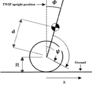
A two wheeled inverted pendulum (TWIP) mobile robot as shown in Fig. 1 is a mechanical system with nonlinear dynamics. It has three degrees of freedom but only two wheels are controlled by the two motors to control all the degrees of motion [1]. It has the advantage of turning on the spot [2] and due to its small body, the robot can enter to the place where the conventional four wheels vehicle cannot.

Accurate model of systems is required to design a controllers especially if the controllers are model based controllers [3]. Many researchers have worked on modelling and control of the TWIP mobile robot. Euler Lagrange methods are implemented in [1, 2, 4, 5], Newton-Euler equations of motion method is used in [6, 7]. In [8, 9] the modelling of TWIP is carried out using Kane’s method of modelling. A Takagi–Sugeno (TS) fuzzy model was used in [10]. All models developed using the various methods were able to emulate the dynamics characteristics of the TWIP to some extent, the Kane’s method gives best model presentation.

In the control of TWIP tilt balancing and position and velocity tracking, linear and non-linear controllers were used extensively, [1, 2, 9, 11, 12]. In [1] linear quadratic regulator (LQR) was developed for balancing and velocity control of the robot, in [2, 9] partial feedback linearization method was employed, pole placement controllers were used in [11, 12]. Combination of LQR and proportional integral derivative (PID) controller was investigated in [13], also a multi operating point model based control using pole placement is presented in

[14]. These linear controllers performed well within the operating region that they are linearized, and also provide acceptable results in other regions but they operating ranges are restricted.

To overcome the restrictions of linear controllers, other controllers apart from linear were also presented in literature

[15-17], in [15] three fuzzy logic controllers (FLC) were proposed based on TS fuzzy and Mamdani architectures for balancing the robot. An adaptive control was implemented in [16] using neural network for balancing the robot, in [17] adaptive and robust controllers were presented. All these controllers give desired results.

In [18], a FLC and PID controller for balancing the robot was presented and compared. The FLC performed better in terms of settling time and less overshoot, while the PID had shown to have better performance in terms of steady state error and rise time. In Partial feedback linearization (PFL) and LQR control schemes, the comparison made in [9], had shown that the LQR controller performed better than the PFL controller in terms of settling time, percent overshoot and the required starting torque, while the PFL controller performed better in terms of rise time. Comparative assessment between LQR and PID-PID scheme was investigated where LQR controller had shown better performance as compared to PID in [19].

Based on this, the performance of a linear and model based controller LQR, a non-model based intelligent controller fuzzy logic and a conventional PID controller, will be assessed experimentally in balancing the TWIP mobile robot. The rest of the paper is organized as follows; section 2 describes the modelling of the robot, section 3 describes the design of the controllers, section 4 give the explanation on the experimental setup, section 5 includes the experimental results and the

International Journal of Mechanical & Mechatronics Engineering IJMME-IJENS Vol:14 No:03 63

146003-8383-IJMME-IJENS © June 2014 IJENS _{I J E N S} performance comparison of the controllers and finally, section

6concludes the findings of this work.

2. MODELLING OF THE TWIP

In this section, the dynamic modelling of the TWIP is presented. Euler Lagrange method is used to derive the dynamic model. The TWIP is modelled as shown in Fig. 2, with parameters shown in Table 1. The TWIP is assumed to have 3 degrees of freedom, x transitional motion, tilt angle, and yaw angle. From the general Langrage formula

Where: T = Total kinetic energy of the system, V = Total potential energy of the system.

Table I

TWIP parameters and variables

PARAMETER Symbol VALUE UNITS

Mass of main body Mb 13. 3 kg

Mass of each wheel Mw 1.89 kg

Center of mass (gravity) from base d 0.13 m

Diameter of wheel R 0.130 m

Distance between the wheels L 0.325 m

Moments of inertia of body wrt x-axis Ix 0.1935 kgm2

Moments of inertia of body wrt z-axis Iz 0.3379 kgm2

Moments of inertia of wheel about the center Ia 0.1229 kgm2

Acceleration due to gravity g 9.81 ms-2

( ̇)

Where = Forced Function, is generalized co-ordinates. For the TWIP, we have 2 inputs torques to motors controlled by voltage.

Total kinetic energy for the TWIP is given in Eq. (3)

Where;

=Body transitional motion = Body rotational motion = Wheel transitional motion = Wheel rotational motion

For : Linear transitional motion =

: Arc distance for x component = : Arc distance for component =

: From general formula of torque, ⁄

Where I =inertia, = angular velocity

⁄ [ ̇ ̇ ̇ ]

For wheel:

⁄ ( ̇ ̇ ₎ ⁄ ( ̇ ̇ )

But , . Substituting these equations in Eq. (5);

( ) ( ̇ ̇ )

Total potential energy V, is given by Eq. (7)

From Eq. (1)

* + ̇ * + ̇ [( ) ( )] ̇ ̇ ̇

Considering x axis:

(

̇) *

+ ̇ ̇

(

̇) *

+ ̈ ̇ ̈

And from Eq. (2)

* + ̈ ̇ ̈

146003-8383-IJMME-IJENS © June 2014 IJENS _{I J E N S} From Eq. 10:

̈ ̈+ ̇ [

]

For coordinate: The Lagrangian is in Eq. (12)

̈ ̈ [ ] ̇

Substitute Eq. 11 in 12 for ̈ and make ̈ the subject of the formula

̈ *( ) + ̇

[ ] * +

* +

Where [

] which becomes

After simplification:

̈ ( )

̇

̇

For x coordinate: From Eq. (8)

̈ *

_{̇ ( )+ ̈}

Substitute Eq. (16) in Eq. (12)

*

̇ ( )+ ̈

̈ [ ] ̇

Now combining the terms with ̈ and making it the subject of the formula yields

̈ ( )

̇

̇

For coordinate: The Lagrangian is given in Eq. (19);

[ ( ) ] ̈ [ ] ̇ ̇

̈

* ( ) +

[ ] ̇ ̇

* ( ) +

International Journal of Mechanical & Mechatronics Engineering IJMME-IJENS Vol:14 No:03 65

146003-8383-IJMME-IJENS © June 2014 IJENS _{I J E N S} To linearize the non-linear model we assume the operating point to be where the tilt angle . Hence ,

, ̇ , ̇ . Therefore Eq. 15, 18, and 20 becomes;

̈

̈

̈

* ( ) +

Substituting the values from the robot parameters shown in Table 1, Eq. 21-23 becomes;

̈ ̈ ̈

In state-space form;

[

]

[

]

Where ̇ ̇ ̇

Eq. 15, 18, and 20 are the dynamical model equations of the TWIP derived using Euler Lagrange method.

3. CONTROLLERS DESIGN

This section describes the detail design of control strategies for model based state feedback LQR controller, non-model based fuzzy logic controller and conventional PID controller for balancing the TWIP robot.

a. State feedback LQR controller

This type of controller uses linear mathematical model of a system in state-space form. An optimal linear quadratic regulator (LQR) estimate the controllers gain using system model [20]. The aim of the controller is to minimize the cost function;

∫

Q is a positive-definite (or positive-semi definite) Hermitian and real symmetric matrix and R is a positive-definite Hermitian and real symmetric matrix.

For the TWIP mobile robot the linearized model is given in Eq. (27) which comprises all the six states of the robot. For this controller design, only four states will be considered, the yaw angle and the velocity of the yaw angle will be neglected. The control scheme is as presented in [1]. Therefore the linearize model is given by Eq. (29)

[

]

[

]

The gain _{of the control law is obtained} by application of the performance index of Eq. (28), and using the solution of algebraic Riccati equation given in Eq. (30)

After experimental tunings the Q and R were found to be, Q =

diag(20 0.1 15 0.1) and R = 5. The controller gain K is computed using MATLAB as

b. Fuzzy Logic controller

A fuzzy logic is a metaheuristic technique, it is used as a control algorithm based on a linguistic control strategy, and does not need any mathematical model [21]. While the others control system use model to provide a controller for the plant, it only uses simple mathematical calculation to simulate the expert knowledge. A Fuzzy logic controller design involves the following:

i. Selection of type and number of membership function. ii. Selection of rule base.

iii. Inference mechanism and, iv. Defuzzification process.

146003-8383-IJMME-IJENS © June 2014 IJENS _{I J E N S}

Table II Fuzzy Rule Base

̇ NB NM NS ZE PS PM PB

NB NB NB NB NB NM NS ZE

NM NB NB NB NM NS ZE PS

NS NB NB NM NS ZE PS PM

ZE NB NM NS ZE PS PM PB

PS NM NS ZE PS PM PB PB

PM NS ZE PS PM PB PB PB

PB ZE PS PM PB PB PB PB

a. PID controller

A PID control scheme is shown in Fig. 3. It is a feedback controller which output (the control variable), is based on the error between defined set point and some measured process variable. The defined set point is tilt angle, which is equal to zero, and the measured process variable is the measured tilt angle from sensors.

The error is fed via elements which perform different actions on the error. Constant KP is multiplied by the error, KI by the

integral of the error, and KD by the derivative of the error. The sum of these 3 signals is the output control signal. The controller parameters were tuned via experiments, and were determined as KP = -10, KI = -0.7, KD = -2 to give the best result.

4. EXPERIMENTAL SETUP

This section explains the experimental setup of the two wheeled inverted pendulum mobile robot. Its schematic overview is shown in Fig. 4.

The TWIP mobile robot is driven by two DC motors, which is driven by a 24v motor driver. The designed controller is implemented on a host PC using MATLAB and Simulink, with Fio Std board microcontroller as the data accusation device [22] . In order to obtain the horizontal displacement of the robot for feedback control, two optical encoder with a resolution of 500 pulses/rev is attached to the shaft of each DC motor [23]. The quadrature encoder signals generated by the optical encoders attached to the motors are connected to Fio Std board which are fed to the host PC for converting pulse to direction in meters, the derivative of the directions is the measured velocity of the mobile robot. [24]. PWM signals are generated according to the designed control law and also supplied to PWM driver via the Fio microcontroller that drive each dc motor. A current sensor [25] is used to measure the current consumed by the motors.

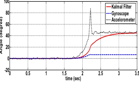
To measure the tilt angle and tilt rate, gyroscope and accelerometer [26] were used. The gyroscope was used to measure angular speed hence the tilt angle is calculated from the data. The gyroscope had the problem of offset, which is a deviation from the measured angular speed. The gyro offset causes a cumulative error over time due to the integral action done in order to obtain the tilt angle. On the other hand, the accelerometer gives the measure of the angle as a function of the static acceleration due to gravity. It has the problem of high levels of noise as a result to the dynamic acceleration when the robot moves horizontally. To overcome the two short comings, the two sensors are used simultaneously using Kalman filter. The outputs of the gyroscope, accelerometer and Kalman filter is shown in Fig. 5.

The gyroscope measures tilt rate directly, inside the MATLAB program the integral of the output is read and is use as the input to Kalman filter subroutine together with accelerometer angle reading, the output of the two gives better accurate result of the tilt angle.

5. RESULT AND DISCUSSION

The performances of the controllers to balance the TWIP mobile robot are presented in this section.

Fig. 4. Experimental block diagram Fig. 3. PID controller and plant

0 0.5 1 1.5 2 2.5 3 3.5

-20 0 20 40 60 80 100

time (sec)

A

n

g

l

e

(d

eg

r

ee)

Tilt Position for 3 Controllers

Kalmal Filter Gyroscope Accelorometer

International Journal of Mechanical & Mechatronics Engineering IJMME-IJENS Vol:14 No:03 67

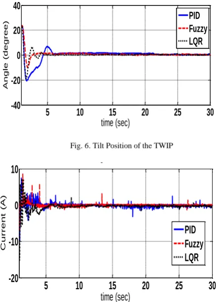
146003-8383-IJMME-IJENS © June 2014 IJENS _{I J E N S} Fig. 6 shows the tilt angle response of the robot. The robot

was initially at 24 degrees; the performance of each controller in balancing the robot is shown. The PID controller has more overshoot than the other controllers and has the slowest settling time. The robot moves 23cm when trying to stabilize in the upright position, while LQR displace the robot about 20cm maximum, and FLC has the less horizontal movement. This is

observed in Fig. 7. Finally Fig. 8 shows the current, which serves as the torque, needed by the motors to achieve the desired goal. The FLC, which performs better than the other two, consumes more energy than the other controllers.

The comparative assessment for the three controllers is summarized in Table III.

Table III

Comparative assessment of controllers

Controllers Rise time (s) Settling time (s)

% Overshoot Current (A)

[Max]

Horizontal

distance

absolute(m)

FLC

1.25

2.5

37

8.7

0.05

LQR

0.8

4.2

80

7.5

0.2

PID

0.8

6.5

90

7.5

0.23

6. CONCLUSION

The dynamical model of a TWIP mobile robot was derived using Euler Lagrange approach. Comparison between model based and non-model base controllers and also conventional PID controller for a balancing the robot is also presented. Practical experiments were carried out to test the controllers and the results are shown and compared. FLC controller which is non-model based performs better than the LQR and PID controllers in terms faster response and less overshoot, but has higher energy consumption than the other two.

ACKNOWLEDGEMENTS

These authors are grateful to the Ministry of Higher

Education (MOHE) and Universiti Teknologi Malaysia for the financial support through the GUP research fund, Vote Q.J130000.2523.05H40 and special thanks to Bayero University, Kano, Nigeria for their support.

REFERENCE

[1] Y. Kim, S. Kim, and Y. Kwak, "Dynamic Analysis of a Nonholonomic Two-Wheeled Inverted Pendulum Robot," Journal

5

10

15

20

25

30

-0.4

-0.2

0

0.2

0.4

time (sec)

m

et

ers

(m

)

Position of Robot

PID

Fuzzy

LQR

5

10

15

20

25

30

-20

-10

0

10

time (sec)

C

urr

en

t

(A)

Control Signal for 3 controllers

PID

Fuzzy

LQR

Fig. 6. Tilt Position of the TWIP

5 10 15 20 25 30

-40 -20 0 20 40

time (sec)

An

gle

(de

gre

e)

Tilt Position for 3 Controllers

PID Fuzzy LQR

Fig. 7. Current consumed by motor

146003-8383-IJMME-IJENS © June 2014 IJENS _{I J E N S}

of Intelligent and Robotic Systems, vol. 44, pp. 25-46, 2005/09/01

2005.

[2] K. Pathak, J. Franch, and S. K. Agrawal, "Velocity and position control of a wheeled inverted pendulum by partial feedback linearization," Robotics, IEEE Transactions on, vol. 21, pp. 505-513, 2005.

[3] A. Calanca, L. M. Capisani, A. Ferrara, and L. Magnani, "MIMO Closed Loop Identification of an Industrial Robot," Control Systems

Technology, IEEE Transactions on, vol. 19, pp. 1214-1224, 2011.

[4] Y.-S. Ha and S. i. Yuta, "Trajectory tracking control for navigation of the inverse pendulum type self-contained mobile robot,"

Robotics and Autonomous Systems, vol. 17, pp. 65-80, 1996.

[5] R. Xiaogang and C. Jing, "B-2WMR System Model and Underactuated Property Analysis," in Automation and Logistics,

2007 IEEE International Conference on, 2007, pp. 580-585.

[6] K. M. Goher, M. O. Tokhi, and N. H. Siddique, "Dynamic Modeling and Control of a Two Wheeled Robotic Vehicle with Virtual Payload," ARPN Journal of Engineering and Applied

Sciences, vol. 6, pp. 7-41, 2011.

[7] L. Jingtao, X. Gao, H. Qiang, D. Qinjun, and D. Xingguang, "Mechanical Design and Dynamic Modeling of a Two-Wheeled Inverted Pendulum Mobile Robot," in Automation and Logistics,

2007 IEEE International Conference on, 2007, pp. 1614-1619.

[8] K. Thanjavur and R. Rajagopalan, "Ease of dynamic modelling of wheeled mobile robots (WMRs) using Kane's approach," in

Robotics and Automation, 1997. Proceedings., 1997 IEEE

International Conference on, 1997, pp. 2926-2931 vol.4.

[9] M. Muhammad, S. Buyamin, M. N. Ahmad, S. W. Nawawi, and Z. Ibrahim, "Velocity Tracking Control of a Two-Wheeled Inverted Pendulum Robot: a Comparative Assessment between Partial Feedback Linearization and LQR Control Schemes," International

Review on Modelling and Simulations, vol. 5, pp. 1038-1048, 2012.

[10] M. Muhammad, S. Buyamin, M. N. Ahmad, and S. W. Nawawi, "Takagi-Sugeno fuzzy modeling of a two-wheeled inverted pendulum robot," Journal of Intelligent & Fuzzy Systems, vol. 25, pp. 535–546, 2013.

[11] F. Grasser, A. D'Arrigo, S. Colombi, and A. C. Rufer, "JOE: a mobile, inverted pendulum," Industrial Electronics, IEEE

Transactions on, vol. 49, pp. 107-114, 2002.

[12] S. W. Nawawi, M. N. Ahmad, and J. H. S. Osman, "Real-time control of a two-wheeled inverted pendulum mobile robot,"

International Journal of mathematical and Computer Sciences, pp.

214-220, 2008.

[13] S. Liang and G. Jiafei, "Researching of Two-Wheeled Self-Balancing Robot Base on LQR Combined with PID," in Intelligent Systems and Applications (ISA), 2010 2nd International Workshop on, 2010, pp. 1-5.

[14] M. Muhammad, S. Buyamin, M. N. Ahmad, S. W. Nawawi, and A. A. Bature, "Multiple Operating Points Model-Based Control of a Two-Wheeled Inverted Pendulum Mobile Robot," International

Journal of Mechanical & Mechatronics Engineering, vol. 13, pp.

1-9, 2013.

[15] H. Cheng-Hao, W.-J. Wang, and C. Chih-Hui, "Design and Implementation of Fuzzy Control on a Two-Wheel Inverted Pendulum," Industrial Electronics, IEEE Transactions on, vol. 58, pp. 2988-3001, 2011.

[16] T. Ching-Chih, H. Hsu-Chih, and L. Shui-Chun, "Adaptive Neural Network Control of a Self-Balancing Two-Wheeled Scooter,"

Industrial Electronics, IEEE Transactions on, vol. 57, pp.

1420-1428, 2010.

[17] L. Zhijun and L. Jun, "Adaptive Robust Dynamic Balance and Motion Controls of Mobile Wheeled Inverted Pendulums," Control

Systems Technology, IEEE Transactions on, vol. 17, pp. 233-241,

2009.

[18] A. N. K. Nasir, M. A. Ahmad, R. Ghazali, and N. S. Pakheri, "Performance Comparison between Fuzzy Logic Controller (FLC) and PID Controller for a Highly Nonlinear Two-Wheels Balancing Robot," in Informatics and Computational Intelligence (ICI), 2011

First International Conference on, 2011, pp. 176-181.

[19] A. N. K. Nasir, M. A. Ahmad, and R. M. T. R. Ismail, "The Control of a Highly Nonlinear Balancing Robot: A Comparative Assessment between LQR and PID-PID Control Schemes,"

International Journal of Computer and Communication

Engineering, pp. 227-232, 2010.

[20] N. S. Nise, Control Systems Engineering, 6 ed.: John Wiley & Sons, Inc, 2011.

[21] S. R. Khuntia, K. B. Mohanty, S. Panda, and C. Ardil, "A Comparative Study of P-I, I-P, Fuzzy and Neuro-Fuzzy Controllers

for Speed Control of DC Motor Drive," International Journal of

Electrical and Computer Engineering, vol. 5, pp. 287-291, 2010.

[22] Microcontroller. (2010, 10/09/2013). FiO Std Datasheet Available:

http://site.gravitech.us/DevelopmentTools/Matlab-Simulink/FiO-Std/fiostdv20_datasheet.pdf

[23] Cytron. (2010). B016 Rotary Encoder. Available:

www.cytron.com.my/viewProduct.php?pcode=B-106-23983‎

[24] Cytron. (2011). MDS40A SmartDrive40. Available:

www.cytron.com.my/viewProduct.php?pcode=MDS40A‎

[25] I. Allegro MicroSystems. (2011). ACS756 Current Sensor IC. Available: www.allegromicro.com