A Partial Least Squares based algorithm for parsimonious variable selection

R E S E A R C H

Open Access

A Partial Least Squares based algorithm for

parsimonious variable selection

Tahir Mehmood

, Harald Martens

, Solve Sæbø

, Jonas Warringer

and Lars Snipen

Abstract

Background:In genomics, a commonly encountered problem is to extract a subset of variables out of a large set of explanatory variables associated with one or several quantitative or qualitative response variables. An example is to identify associations between codon-usage and phylogeny based definitions of taxonomic groups at different taxonomic levels. Maximum understandability with the smallest number of selected variables, consistency of the selected variables, as well as variation of model performance on test data, are issues to be addressed for such problems.

Results:We present an algorithm balancing the parsimony and the predictive performance of a model. The algorithm is based on variable selection using reduced-rank Partial Least Squares with a regularized elimination. Allowing a marginal decrease in model performance results in a substantial decrease in the number of selected variables. This significantly improves the understandability of the model. Within the approach we have tested and compared three different criteria commonly used in the Partial Least Square modeling paradigm for variable selection; loading weights, regression coefficients and variable importance on projections. The algorithm is applied to a problem of identifying codon variations discriminating different bacterial taxa, which is of particular interest in classifying metagenomics samples. The results are compared with a classical forward selection algorithm, the much used Lasso algorithm as well as Soft-threshold Partial Least Squares variable selection.

Conclusions:A regularized elimination algorithm based on Partial Least Squares produces results that increase understandability and consistency and reduces the classification error on test data compared to standard approaches.

Background

With the tremendous increase in data collection techni-ques in modern biology, it has become possible to sam-ple observations on a huge number of genetic, phenotypic and ecological variables simultaneously. It is now much easier to generate immense sets of raw data than to establish relations and provide their biological interpretation [1-3]. Considering cases of supervised sta-tistical learning, huge sets of measured/collected vari-ables are typically used as explanatory varivari-ables, all with a potential impact on some response variable, e.g. a phe-notype or class label. In many situations we have to deal with data sets having a large number of variablesp in comparison to the number of samplesn. In such‘large

psmall n’ situations selection of a smaller number of influencing variables is important for increasing the per-formance of models, to diminish the curse of dimen-sionality, to speed up the learning process and for interpretation purposes [4,5]. Thus, some kind of vari-able selection procedure is frequently needed to elimi-nate unrelated features (noise) for providing a more observant analysis of the relationship between a modest number of explanatory variables and the response. Examples include the selection of gene expression mar-kers for diagnostic purposes, selecting SNP marmar-kers for explaining phenotype differences, or as in the example presented here, selecting codon preferences discriminat-ing between different bacterial phyla. The latter is parti-cularly relevant to the classification of samples in metagenomic studies [6]. Multivariate approaches like correspondence analysis and principal component analy-sis has previously been used to analyze variations in * Correspondence: tahir.mehmood@umb.no

1

Biostatistics, Department of Chemistry, Biotechnology and Food Sciences, Norwegian University of Life Sciences, Norway

Full list of author information is available at the end of the article

codon usage among genes [7]. However, in order to relate the selection specifically to a response vector, like the phylum assignment, we need a selection based on a supervised learning method.

Partial Least Square (PLS) regression is a supervised method specifically established to address the problem of making good predictions in the‘largepsmalln’ situa-tion, see [8]. PLS in its original form has no implemen-tation of variable selection, since the focus of the method is to find the relevant linear subspace of the explanatory variables, not the variables themselves. However, a very large pand smallncan spoil the PLS regression results, as demonstrated by Keles et. al.[9], discovering that the asymptotic consistency of the PLS estimators for univariate responses do not hold, and by [10], who observed a large variation on test set.

Boulesteix has theoretically explored a tight connec-tion between PLS dimension reducconnec-tion and variable selection [11] and work in this field has existed for many years. Examples are [8,9,11-23]. For an optimum extraction of a set of variables, we need to look for all possible subsets of variables, which is impossible ifpis large enough. Normally a set of variables with a reason-able performance is a compromise over the optimal sub set.

In general, variable selection procedures can be cate-gorized [5] into two main groups: filter methods and wrapper methods. Filter methods select variables as a preprocessing step independently of some classifier or prediction model, while wrapper methods are based on some supervised learning approach [12]. Hence, any PLS-based variable selection is a wrapper method. Wrapper methods need some sort of criterion that relies solely on the characteristics of the data as described by [5,12]. One candidate among these criteria is the PLS loading weights, where down-weighting small PLS loading weights is used for variable selection [8,11,13-17,24-27]. A second possibility is to use the magnitude of the PLS regression coefficients for variable selection [18-20,28-34]. Jackknifing and/or bootstrapping on regression coefficients has been utilized to select influencing variables [20,30,31,33,34]. A third commonly used criterion is the Variables Importance on PLS pro-jections (VIP) introduced by Erikssonet. al.[21] and is commonly used in practise [22,31,35-37].

There are several PLS-based wrapper selection algo-rithms, for example uninformative variable elimination (UVE-PLS) [18], where artificial random variables are added to the data as a reference such that the variable with least performance are eliminated. Iterative PLS (IPLS) adds new variable(s) in the model or remove variables from the model if it improves the model per-formance [19]. A backward elimination procedure based

on leave one variable out is another example [5]. Although wrapper based methods perform well the number of variables selected is still often large [5,12,38], which may make interpretation hard ([23,39,40]).

Among recent advancements in PLS methodology itself we find that Indahlet. al.[41] propose a new data compression method for estimating optimal latent vari-ables classification and regression problems by combin-ing PLS methodology and canonical correlation analysis (CCA), called Canonical Powered PLS (CPPLS). In our work we have adopted this new methodology and pro-posed a regularized greedy algorithm based on a back-ward elimination procedure. The focus is on classification problems, but the same concept can be used for prediction problems as well. Our principle idea is to focus on a parsimonious selection, achieved by tol-erating a minor performance deviation from any‘ opti-mum’if this gives a substantial decrease in the number of selected variables. This is implemented as a regulari-zation of the search for optimum performance, making the selection less dependent on‘peak performance’and hence more stable. In this respect, the choice of the CPPLS variant is not important, and even the use of non-PLS based methods could in principle be imple-mented with some minor adjustments. Both loading weights, PLS regression coefficients significance obtained from jackknifing and VIP are explored here for ordering the variables with respect to their importance.

1 Methods

1.1 Model fitting

We consider a classification problem where every object belongs to one out of two possible classes, as indicated by then× 1 class label vector C. FromCwe create the

n× 1 numeric response vectory by dummy coding, i.e. y contains only 0’s and 1’s. The association betweeny and the n × p predictor matrix X is assumed to be explained by the linear model E(y) =Xbwherebare the

p× 1 vector of regression coefficients. The purpose of variable selection is to find a column subset of X cap-able of satisfactory explaining the variations inC.

From a modeling perspective, ordinary least square fit-ting is no option when n <p. PLS resolves this by searching for a small set of components,‘latent vectors’, that performs a simultaneous decomposition of Xandy with the constraint that these components explain as much as possible of the covariance betweenXandy.

1.2 Canonical Powered PLS (CPPLS) Regression

ˆ

β=Wˆ(Pˆ₁Wˆ)−1pˆ₂ (1)

where Pˆ1is the pl × k matrix of X-loadings that is

summary of X-variables,pˆ2is the avector ofy-loadings

i.e. summary of y-variables and_Wˆ is thep×kmatrix of loading weights, for details see [8]. Recently, Indahlet. al.[41] proposed a new data compression method for estimating optimal latent variables by combining PLS methodology and canonical correlation analysis (CCA). They introduce a flexible trade-off between the element wise correlations and variances specified by a power parameter g, ranging from 0 to 1. Defines the loading weights as

w(γ) =Kγ ⎡ ⎣s1|corr(x1,y)|

γ

1−γ .std(x1)

1−γ γ , ...,

sp|corr(xp,y)|

γ

1−γ.std(xp)

1−γ γ

⎤ ⎥ ⎦

t

whereskdenotes the sign of thekth correlation andKg

is a scaling constant assuring unit length w(g). In this study we restrictedgto lower region (0.001, 0.050) and to upper region (0.950, 0.999). This means we consider combinations ofgfor emphasizing either the variance (g close to 0) or the correlations (gclose to 1). Thegvalue from above regions that optimizes the canonical correla-tion is always selected for each component of CPPLS algorithm, see Indahl et. al. [41] for details on the CPPLS algorithm.

Based on the CPPLS estimated regression coefficients

ˆ

βwe can predict the dummy-variables by

ˆ y=Xβˆ

and from the data set(yˆ,C)we build a classifier using straightforward linear discriminant analysis [42].

1.3 First regularization - model dimension estimate

The CPPLS algorithm assumes that the column space of Xhas a subspace of dimensionacontaining all informa-tion relevant for predicting y (known as the relevant subspace) [43]. In order to estimateawe use cross-vali-dation and the performancePadefined as the fraction of

correctly classified observations in a cross-validation procedure, usingacomponents in the CPPLS algorithm. The cross-validation estimate ofa can be found by systematically trying out a range of dimensionsa= 1,...,

A, computePafor eacha, and choose as αˆ theawhere

we reach the maximumPa. Let us denote this valuea*.

It is well known that in many cases Pawill be almost

equally large for many choices ofa. Thus, estimating a by this maximum value is likely to be a rather unstable estimator. To stabilize this estimate we use a regulariza-tion based on the principle of parsimony where we

search for the smallest possibleawhose corresponding performance is not significantly worse than the opti-mum. If rais the probability of a correct classification

using the a-component model, and ra* similar for the

a*-component model, we testH0 : ra=ra* against the

alternative H1 :ra<ra*. In practicePaandPa* are

esti-mates of raand ra*. The smallest awhere we cannot

reject H0 is our estimateαˆ. The testing is done by

ana-lyzing the 2 × 2 contingency table of correct and incor-rect classifications for the two choices of a, using the McNemar test [44]. This test is appropriate since the model classification at a specific component depends on the model classification at the other components.

This regularization depends on a user-defined rejec-tion levelc of the McNemar test. Using a largec(close to 1) means we easily reject H0, and the estimate αˆ is

often similar toa*. By choosing a smallerc(closer to 0) we get a harder regularization, i.e. a smaller_αˆ and more stability at the cost of a lower performance.

1.4 Selection criteria

We have implemented and tried out three different cri-teria for PLS-based variable selection:

1.4.1 Loading weights

Variable j can be eliminated if the relative loading weight, rj for a given PLS component satisfies

rj=|

wa,j

maxwa|<

ufor some chosen thresholduÎ [0, 1].

1.4.2 Regression coefficients

Variablejcan be eliminated if the corresponding regres-sion coefficientbj= 0. Testing H0 :bj= 0 againstH1:bj

≠= 0 can be done by a jackknife t-test. All computa-tions needed have already been done in the cross-valida-tion used for estimating the model dimension a. For each variable we compute the corresponding false dis-covery rate (q -value) which is based on the pvalues from jackknifing, and variable jcan be eliminated ifqj

>ufor some fixed thresholduÎ[0, 1].

1.4.3 Variable importance on PLS projections (VIP)

VIP for the variable jis defined according to [21] as

vj=

p

a∗

a=1 [(p2

2atata)(waj/||wa||)2]/ a∗

a=1 (p2

2a(tata)

where a = 1, 2, ..., a*, waj is the loading weight for

variable j using acomponents and ta, wa and p2aare

CPPLS scores, loading weights andy-loadings respec-tively corresponding to theathcomponent. [22] explains the main difference between the regression coefficientbj

andvj. Thevjweights the contribution of each variable

according to the variance explained by each PLS compo-nent, i.e. p2

2atata where (waj/||wa||)2 represents the

eliminated ifvj<ufor some user-defined thresholduÎ

[0, ∞). It is generally accepted that a variable should be selected if vj> 1, see [21,22,36], but a proper

thresh-old between 0.83 and 1.21 can maximize the perfor-mance [36].

1.5 Backward elimination

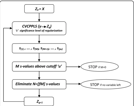
When we haven<<pit is very difficult to find the truly influencing variables since the estimated relevant sub-space found by Cross-Validated CPPLS (CVCPPLS) is bound to be, to some degree, ‘infested’by non-influen-cing variables. This may easily lead to errors both ways, i.e. both false positives and false negatives. An approach to improve on this is to implement a stepwise estima-tion where we gradually eliminate ‘the worst’ variables in a greedy algorithm.

The algorithm can be sketched as follows: LetZ0=X

and let sj be one of the criteria for variablej we have

sketched above (eitherrj,qjorvj).

1) For iteration g runy andZgthrough CVCPPLS.

The matrix Zghas pgcolumns, and we get the same

number of criterion values, sorted in ascending order as s(1), ...,s(pg).

2) There are M criterion values below (above for citerion qj) the cutoff u. If M = 0, terminate the

algorithm here.

3) Else, let N = ⌈fM⌉ for some fraction f Î 〈0,1]. Eliminate the variables corresponding to the Nmost extreme criterion values.

4) If there are still more than one variable left, let Zg

+1contain these variables, and return to 1).

The fractionfdetermines the‘steplength’of the elimi-nation algorithm, where anfclose to 0 will only elimi-nate a few variables in every iteration. The fraction f

anducan be obtained through cross validation.

1.6 Second regularization - final selection

In each iteration of the elimination the CVCPPLS algo-rithm computes the cross-validated performance, and we denote this withPgfor iteration g. After each

itera-tion, the number of influencing variables decreases, but

Pgwill often increase until some optimum is achieved,

and then drop again as we keep on eliminating. The initial elimination of variables stabilizes the estimates of the relevant subspace in the CVCPPLS algorithm, and hence we get an increase in performance. Then, if the elimination is too severe, we start to lose informative variables, and even if stability is increased even more, the performance drops.

Let the optimal performance be defined as

P∗=Pg∗ = max g Pg

It is not unreasonable to use the variables still present after iteration g* as the final selected variables. This is where we have achieved a balance between removing noise and keeping informative variables. However, fre-quently we observe that a severe reduction in the num-ber variables compared to this‘optimum’will give only a modest drop in performance. Hence, we may eliminate well beyond g*, and find a much simpler model, at a small loss in performance. To formalize this, we use exactly the same procedure, involving the McNemar test that we used in the regularization of the model dimen-sion estimate. Ifrgis the probability of a correct

classifi-cation after g iterations, and rg* similar after g*

iterations, we test H0 : rg =rg* against the alternative

H1 :rg<rg*. The largestgwhere we cannot reject H0is

the iteration where we find our final selected variables. This means we need another rejection leveldwhich will decide to which degree we are willing to sacrifice perfor-mance over a simpler model. Usingdclose to 0 means we emphasize simplicity over performance. In practice, for each iteration beyondg* we can compute the McNe-mar testp-value, and list this together with the number of variables remaining, to give a perspective on the trade-off between understandability of the model and the performance. Figure 1 presents the procedure in a flow chart.

1.7 Choices of variable selection methods for comparison

Three variable selection methods are also considered for comparison purposes. The classical forward selection

Z0 = X

CVCPPLS (y Zg) ‘c’ significance level of regularization

s(1) , ... , s(M), s(M+1), ... , s(pg)

M s-values above cutoff ‘u’ STOP if M=0

Eliminate N=[fM] s-values STOP if no variable left

Zg+1

Figure 1Flow chart. The flow chart illustrates the proposed

procedure (Forward) is a univariate approach, and prob-ably the simplest approach to variable selection for the ‘large p small n’type of problems considered here. The Least Absolute Shrinkage and Selection Operator (Lasso) [45] is a method frequently used in genomics. Recent examples are the extraction of molecular signa-tures [46] and gene selection from microarrays [47]. The Soft-Thresholding PLS (ST-PLS) [17] implements the Lasso concept in a PLS framework. A recent application of ST-PLS is the mapping of genotype to phenotype information [48].

All methods are implemented in the R computing environment http://www.r-project.org/.

2 Application

An application of the variable selection procedure is to find the preferred codons associated with certain pro-karyotic phyla.

Codons are triplets of nucleotides in coding genes and the messenger RNA; these triplets are recognized by base-pairing by corresponding anticodons on specific transfer RNA carrying individual amino acids. This facil-itates the translation of genetic messenger information into specific proteins. In the standard genetic code, the 20 amino acids are individually coded by 1, 2, 4 or 6 dif-ferent codons (excluding the three stop codons there are 61 codons). However, the different codons encoding individual amino acids are not selectively equivalent because the corresponding tRNAs differ in abundance, allowing for selection on codon usage. Codon preference is considered as an indicator of the force shaping gen-ome evolution in prokaryotes [49,50], reflection of life style [49] and organisms within similar ecological envir-onments often have similar codon usage pattern in their genomes [50,51]. Higher order codon frequencies, e.g. di-codons, are considered important with respect to joint effects, like synergistic effect, of codons [52].

There are many suggested procedures to analyze codon usage bias, for example the codon adaptation index [53], the frequency of optimal codons [54] and the effective number of codons [55]. In the current study, we are not specifically looking at codon bias, but how the overall usage of codons can be used to distin-guish prokaryote phyla. Notice that the overall codon usage is affected both by the selection of amino acids and codon bias within the redundant amino acids. Phy-lum is a relevant taxonomic level for metagenomic stu-dies [56,57], so interest lies in having a systematic search for codon usage at the phylum level [58-60].

2.1 Data

Genome sequences for 445 prokaryote genomes and the respective Phylum information were obtained from NCBI Genome Projects (http://www.ncbi.nlm.nih.gov/

genomes/lproks.cgi). The response variable in our data set is phylum, i.e. the highest level taxonomic classifier of each genome, in the bacterial kingdom. There are in total 11 several phyla in our data set including Actino-bacteria, Bacteroides, Crenarchaeota, Cyanobac-teria,

Euryarchaeota, Firmicutes,Alphaproteobacteria, Beta-proteobacteria, Deltaproteobacteria, Gammapro-teobac-teriaandEpsilonproteobacteria. We only consider two-class problems, i.e. for some fixed ‘phylum A’, we only classify genomes as either ‘phylum A’, or ‘not phylum A’. Thus, the data set has n= 445 samples and 11 dif-ferent responses of 0/1 outcome, considering one at a time.

Genes for each genome were predicted by the gene-finding software Prodigal [61], which uses dynamic pro-gramming in which start codon usage, ribosomal site motif usage and GC frame bias are considered for gene prediction. For each genome, we collected the frequen-cies of each codon and each di-codon over all genes. The predictor variables thus consists of relative frequen-cies for all codons and di-codons, giving a predictor matrix Xwith a total of p= 64 + 642 = 4160 variables (columns).

2.2 Parameter setting/tuning

It is in principle no problem to eliminate (almost) all variables, since we always go back to the iteration where we cannot reject the null-hypothesis of the McNemar test. Hence, we fixedu at extreme values, 0.99 for load-ing weights, 0.01 for regression coefficients and 10 for VIP. Three levels of step lengthf= (0.1,0.5, 1) were con-sidered. In the first regularization step we tried three very different rejection levelsc = (0.1,0.5, 1) and in the second we used two extreme levels (d= (0.01,0.99)).

2.3 The split of data into test and training

Figure 2 gives a graphical overview of the data splitting used in this study. The split is carried out at three levels. At level 1 we split the data into a test set containing 25% of the genomes and a training set containing the remaining 75%. This was repeated 100 times, i.e. 100 pairs of test and training sets were constructed by ran-dom drawing with replacement. Test and training set were never allowed to overlap. In each of the 100 instances, the training data were used by each of the four methods listed to the right. They select variables, and the selected variables were used for classifying the level 1 test set, and performance was computed for each method.

level 3 leave-one-out cross-validation was used to esti-mate all parameters in the regularized CPPLS method, including the rejection levelc. These two levels together corresponds to a‘cross-model validation’[62].

3 Results and Discussions

For identification of codon variations that distinguishes different bacterial taxa to be utilized as classifiers in metagenomic analysis, 11 models, representing each phylum, were considered separately. We have chosen the phylum Actinobacteriafor a detailed illustration of the method, while results for all phyla are provided below. In Figure 3 we illustrate how the elimination pro-cess affects model performance (P) reflecting the per-centage of correctly classified samples, starting at the left with the full model and iterating to the right by eliminating variables. Use of any of the three criteria loading weights, regression coefficient significance or VIP, produces the same type of behavior. A fluctuation in performance over iterations is typical, reflecting the noise in the data. At each iteration, we only eliminate a fraction (1% in many cases) of the poor ranking vari-ables, giving the remaining variables a chance to increase the performance at later iterations. We do not stop at the maximum performance, which may occur almost anywhere due to the noise, but keep on eliminat-ing until we reach the minimum model not significantly worse than the best. This may lead to a substantial decrease in the number of variables selected.

In the upper panels of Figure 4, a comparison of the number of variables selected by the ‘optimum’ model and our selected model is displayed. A cross-comparison

of the criteria loading weights, regression coefficient and VIP based elimination procedure is also made. Xiaobo

et. al. [23] has criticized the wrapper procedures for being unable to extract a small number of variables, which is important for interpretation purposes [23,39]. This is reflected here as none of the‘optimum’ model Forward _Lasso

St-PLS Level 1

Test

Train

Stepwise Elimination Level 2

Test

Train

Test

Train CVCPPLS

Stepwise Elimination Level 3

Figure 2An overview of the testing/training. An overview of the testing/training procedure used in this study. The rectangles illustrate the predictor matrix. At level 1 we split the data into a test set and training set (25/75) to be used by all four methods listed on the right. This was repeated 100 times. Inside our suggested method, the stepwise elimination, there are two levels of validation. First a 10-fold cross-validation was used to optimize selection parametersfandd, and at level 3 leave-one-out cross-validation was used to optimize the regularized CPPLS method.

90

91

92

93

Number of variables left in the model

Pe

rf

or

mance

4160 2524 1513 907 596 390 254 166 108 70 45 28 Full Model

Optimum Model

Selected Model

Figure 3A typical elimination. A typical elimination is shown

based on the data for phylumActinobacteria. Each dot in the figure indicates one iteration. The procedure starts on the left hand side, with the full model. After some iterations performance(P), which reflects the percentage of correctly classified samples, has increased, and reaches a maximum. Further elimination reduces performance, but only marginally. When elimination becomes too severe, the performance drops substantially. Finally, the selected model is found where we have the smallest model with performance not

selections (lower boxes) resulted in a small number of selected variables. However, using our regularized algo-rithm (upper boxes) we are able to select a small num-ber of variables in all cases. The VIP based elimination performs best in this respect (upper right panel), but the other criteria are also competing well. The variance in model size is also very small for our regularized algo-rithm compared to the selection based on ‘optimum’ performance.

Comparison of the number of variables selected by Forward, Lasso and ST-PLS is made in the lower panels of Figure 4. All three methods end up with a small number of selected variables on the average, but ST-PLS has a large variation in the number of selected variables.

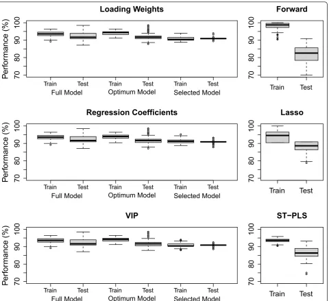
The classification performances in the test and training data sets are examined in Figure 5. In the left panels we show the results for our procedure using the criteria loading weights, regression coefficient and VIP during selection. In general all three criteria behave equally well. As expected, the best performance is found in the train-ing data for the‘optimum’model. Also, performance is

consistently worse in the test data compared to the train-ing data for all cases, but this pattern is most clearly pre-sent for the‘optimum’model. This may be seen as an indication of over-fitting. A huge variation in test data performance can be observed for the full model, and slightly smaller for the‘optimum’model. Our selected models give somewhat worse overall training perfor-mance, but evaluated on the test sets they come out at the same level as the‘optimum’model, and with a much smaller variance.

In the right hand panels, performance is shown for the three alternative methods. Our algorithm comes out with at least as good performance on the test sets as any of the three alternative methods. Particularly notably is the larger variation in test performance for the alter-native methods compared to the selected models in the left panels. A formal testing by the Mann-Whitney test [63] indicates that our suggested procedure with VIP outperforms Lasso (p< 0.001), Forward (p< 0.001) and ST-PLS (p< 0.001) on the data sets used in this study. The same was also true if we used loading weights or regression coefficient as ranking criteria.

0 20 40 60 80

Loading Weights

Relative Size (%)

Optimum Model

Selected Model

0 20 40 60 80

Regression Coefficients

Relative Size (%)

0 20 40 60 80

VIP

Relative Size (%)

0 20 40 60 80

Forward

Relative Size (%)

Fitted model

0 20 40 60 80

Lasso

Relative Size (%)

0 20 40 60 80

ST

−

PLS

Relative Size (%)

Figure 4The distribution of selected variables. The distribution of the number of variables selected by the optimum model and selected

When we are interested in the interpretation of the variables, it is imperative that the procedure we use shows some stability with respect to which variables are being selected. To examine this we introduce a selectiv-ity score. If a variable is selected as one out of m vari-ables, it will get a score of 1/m. Repeating the selection 100 times for the same variables, but with slightly differ-ent data, we add up the scores for each variable and divide by 100. Thus, a variable having a large selectivity score is often selected as one among a few variables. A procedure that selects almost all variables, or completely

new variables, each time, will produce very similar and small selectivity scores for all variables. Conversely, a procedure that home in on the same few variables in each case, will produce some very big selectivity scores on these variables. In Figure 6 we show the selectivity scores sorted in descending order for the three criteria loading weights, regression coefficients and VIP, and for the alternative methods Forward, Lasso and ST-PLS selection. This indicates that VIP is the most stable cri-terion, giving the largest selectivity scores, but loading weights and regression coefficient performs almost as

70

80

90

100

Loading Weights

Pe

rf

or

mance

(%)

Train Test Train Test Train Test

Full Model Optimum Model Selected Model

70

80

90

100

Regression Coefficients

Pe

rf

or

mance

(%)

Train Test Train Test Train Test

Full Model Optimum Model Selected Model

70

80

90

100

VIP

Pe

rf

or

mance

(%)

Train Test Train Test Train Test

Full Model Optimum Model Selected Model

70

80

90

100

Forward

Train Test

70

80

90

100

Lasso

Train

Test

70

80

90

100

ST

−

PLS

Train

Test

good. The Lasso method is as stable as our proposed method using the VIP criterion, while Forward and ST-PLS seems worse as they spread the selectivity score over many more variables. From the definition of VIP we know that the importance of the variables is down-weighted as number of CPPLS components increases. This probably reduces the noise influence and thus pro-vides more stable and consistent selection, also observed by [22].

95% of our selected model uses 1 component while the rest uses 2 components. It is clear from the defini-tion of Loading weights, VIP and regression coefficients that the sorted index of variables based on these mea-sures will be the same for 1 component. This could be the reason for the rather similar behavior of loading weights, VIP and regression coefficient in above analysis. In order to get a rough idea of the‘null-distribution’ of this selectivity score, we ran the selection on data

0

100 200 300 400 500

0.000

0.025

Loading Weights

Sorted index of variables

S

el

ec

tiv

ity score

0

100 200 300 400 500

0.000

0.025

Forward

Sorted index of variables

S

el

ec

tiv

ity score

0

100 200 300 400 500

0.000

0.025

VIP

Sorted index of variables

S

el

ec

tiv

ity score

0

100 200 300 400 500

0.000

0.025

Lasso

Sorted index of variables

S

el

ec

tiv

ity score

0

100 200 300 400 500

0.000

0.025

Regression Coefficients

Sorted index of variables

S

el

ec

tiv

ity score

0

100 200 300 400 500

0.000

0.025

ST

−

PLS

Sorted index of variables

S

el

ec

tiv

ity score

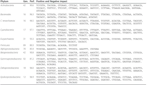
where the response ywas permuted at random. From this the upper 0.1% percentile of the null-distribution is determined, which is approximately corresponds to the selectivity score above 0.01. For each phylum and vari-ables giving a selectivity score above this percentile are listed in Table 1. The selected variables will also have positive or negative impact depending on the sign of the regression coefficients as indicated in the table. A di-codon with a positive/negative regression coefficient is informative because it occurs more/less frequently in this phylum than in the entire population. It appears that, the larger phyla are in general more difficult to classify, simply because there are more diversity inside the group. On the other hand, the results obtained for the larger phyla are more relevant. Because a larger set of genomes usually means less sampling bias, i.e. the data set represents the phylum better. Interestingly, all of the selected variables are di-codons (no single codons), providing additional support for that the inter-action of codons are highly important for explaining variations in phyla [49,52,64]. It should be noted that the performance listed for each phylum in Table 1 is an optimistic estimate of the real performance we must expect on a new data set, since it is based on variables selected by maximizing performance over all data in the

present data set. However, for comparisons between phyla they are still relevant.

4 Conclusion

We have suggested a regularized backward elimination algorithm for variable selection using Partial Least Squares, where the focus is to obtain a hard, and at the same time stable, selection of variables. In our proposed procedure, we compared three PLS-based selection cri-teria, and all produced good results with respect to size of selected model, model performance and selection sta-bility, with a slight overall improvement for the VIP cri-terion. We obtained a huge reduction in the number of selected variables compared to using the models with optimum performance based on training. The apparent loss in performance compared to the optimum based models, as judged by the fit to the training set, is vir-tually disappearing when evaluated on a separate test set. Our selected model performs at least as good as three alternative methods, Forward, Lasso and ST-PLS, on the present test data. This also indicates that the reg-ularized algorithm not only obtain models with superior interpretation potential, but also an improved stability with respect to classification of new samples. A method like this could have many potential uses in genomics,

Table 1 Selectivity score based selected codons

Phylum Gen. Perf. Positive and Negative impact

Actinobacteria 42 90.6 TCCGTA, TACGGA, GTGAAG, CTTCAC, TGTACA, TCCGTT, AGAAGG, CCTTCT, GAGGCT, GGAACA,

TCCACC, TGTTCC, TTCCGT, CTTAAG, GGGATC, GATCCC, CCTTAA, TTAAGG AACGGA, GGTGGA,

GTCGAC,

Bacteroides 16 96.3 TATATA, TCTATA, CTATAT, TATAGA, ATATAG, TATAGT, TTATAG, CTTATA, CTATAA, ACTATA,

TATATC, GATATA, CTATAG, TATACT TATAAG, ATATAT,

C renarchaeota 16 96.5 AACGCT, AGCGTT, ACGAGT, ACTCGT, ACGACT, TTAGGG, TCGTGT, ACACGA, CCCTAA, TAGCGT,

TACGAG, ACGCTA, CGTGTT, AACACG, GGGCTA, CTACGA, TCGTAG, CGAGTA, TACTCG, GCGTTT

AGTCGT, CTCGTA, TAGCCC,

Cyanobacteria 17 97.1 CAATTG, GTTCAA, TTGAAC, TAAGAC, GTCTTA, CTTAGT, TTAGTC, GGTCAA, GACTAA, ACTAAG,

CTTGAT, AAGTCA, ATCAAG, TGGTTC, GAACCA, AGTCAA, GACCAA, TTGGTC, TTGATC, GACTTG,

TCTTAG, CAAGTC TTGACC, TGACTT, TTGACT, GATCAA,

Euryarchaeota 31 93.3 ACACCG, CGGTGT, TCGGGT, GGTGTC, TCGGTG, CACCGA, ACCCGA, CCGCGG, GGTGTG, TCACCG,

TATCGT, TACGCT, TTCTGC GACACC, CACACC,

Firmicutes 89 80.3 _{TCGGTA, TACCGA, ACAGGA, TCCTGT}

Alphaproteobacteria 70 85.9 TCGCGA, AAGATC, GATCTT, TTCGCG, AAATTT, CGCGAA

Betaproteobacteria 42 90.8 GGAACA, TGTTCC, TAGTCG, CGACTA, GCTAGC, AAGCTC, GAGCTT, TACGAG, CTCGTA, CTTGCA,

GATCTT, TGCAAG, AAGATC, AGGCTT, AAGCCT, CTCGAG

Gammaproteobacteria 92 81.2 CTCAGT, ACTGAG, GACTCA, TGAGTC, ACTCAG, ACTCTG, CAGAGT, CTCAGA, TCTGAG, CTGTCT,

CCAGAG, CTCTGG, TCACCT, TGACTC, CTCTGT, AGGTGA, GAGTCA, TCACTC, GAGTGA CTGAGT,

AGACAG, ACAGAG,

Deltaproteobacteria 18 96.0 _{GACATT, TCATGT, ACATGA, AATGTC, AACATC, ATGTTG, CAACAT, CATTGT, ACAATG, ACATTG,}

ACAACA, TGTTGT, AACAAC, GTTGTT, CATTTC, GTTCCA, TGGAAC, CAACAA, TTGTTG, GAAACA,

GGAACA, TGTTCC, AATGAC, GTCATT GATGTT, CAATGT, GAAATG, TGTTTC,

Epsilonproteobacteria 12 96.9 TCCTGT, ACAGGA, GTATCC, TCAGGA, TCCTGA, TGCAGA, TCTGCA, TTCAGG, CCTGAA, ATATCC,

GAACCT, AGGTTC, GGAGAT, ATCTCC, TTGCAG, GGATAC, GGATAT, CTGCAA, TCCCTG, CAGGGA, ACTGCA, TGCAGT, TTCCTG, TACAGG

but more comprehensive testing is needed to establish the full potential. This proof of principle study should be extended by multi-class classification problems as well as regression problems before a final conclusion can be drawn. From the data set used here we find a smallish number of di-codons associated with various bacterial phyla, which is motivated by the recognition of bacterial phyla in metagenomics studies. However, any type of genome-wide association study may potentially benefit from the use of a multivariate selection method like this.

Acknowledgements

Tahir Mehmoods scholarship has been fully financed by the Higher Education Commission of Pakistan, Jonas Warringer was supported by grants from the Royal Swedish Academy of Sciences and Carl Trygger Foundation.

Author details

1_{Biostatistics, Department of Chemistry, Biotechnology and Food Sciences,}

Norwegian University of Life Sciences, Norway.2_{Centre of Integrative}

Genetics (CIGENE), Animal and Aquacultural Sciences, Norwegian University of Life Sciences, Norway.3_{Department of Cell- and Molecular Biology,}

University of Gothenburg, Sweden.

Authors’contributions

TM and LS initiated the project and the ideas. All authors have been involved in the later development of the approach and the final algorithm. TM has done the programming, with some assistance from SS and LS. TM and LS has drafted the manuscript, with inputs from all other authors. All authors have read and approved the final manuscript.

Competing interests

The authors declare that they have no competing interests.

Received: 28 September 2011 Accepted: 5 December 2011 Published: 5 December 2011

References

1. Bachvarov B, Kirilov K, Ivanov I:Codon usage in prokaryotes.Biotechnology and Biotechnological Equipment2008,22(2):669.

2. Binnewies T, Motro Y, Hallin P, Lund O, Dunn D, La T, Hampson D, Bellgard M, Wassenaar T, Ussery D:Ten years of bacterial genome sequencing: comparative-genomics-based discoveries.Functional & integrative genomics2006,6(3):165-185.

3. Shendure J, Porreca G, Reppas N, Lin X, McCutcheon J, Rosenbaum A, Wang M, Zhang K, Mitra R, Church G:Accurate multiplex polony sequencing of an evolved bacterial genome.Science2005, 309(5741):1728.

4. Hastie T, Tibshirani R, Friedman J:The Elements of Statistical Learning. 2008.

5. Fernández Pierna J, Abbas O, Baeten V, Dardenne P:A Backward Variable Selection method for PLS regression (BVSPLS).Analytica chimica acta

2009,642(1-2):89-93.

6. Riaz K, Elmerich C, Moreira D, Raffoux A, Dessaux Y, Faure D:A metagenomic analysis of soil bacteria extends the diversity of quorum-quenching lactonases.Environmental Microbiology2008, 10(3):560-570.

7. Suzuki H, Brown C, Forney L, Top E:Comparison of correspondence analysis methods for synonymous codon usage in bacteria.DNA Research

2008,15(6):357.

8. Martens H, Næs T:Multivariate CalibrationWiley; 1989.

9. KeleşS, Chun H:Comments on: Augmenting the bootstrap to analyze high dimensional genomic data.TEST2008,17:36-39.

10. Höskuldsson A:Variable and subset selection in PLS regression. Chemometrics and Intelligent Laboratory Systems2001,55(1-2):23-38.

11. Boulesteix A, Strimmer K:Partial least squares: a versatile tool for the analysis of high-dimensional genomic data.Briefings in Bioinformatics

2007,8:32.

12. John G, Kohavi R, Pfleger K:Irrelevant features and the subset selection problem.InProceedings of the eleventh international conference on machine learning. Volume 129.Citeseer; 1994:121-129.

13. Jouan-Rimbaud D, Walczak B, Massart D, Last I, Prebble K:Comparison of multivariate methods based on latent vectors and methods based on wavelength selection for the analysis of near-infrared spectroscopic data.Analytica Chimica Acta1995,304(3):285-295.

14. Alsberg B, Kell D, Goodacre R:Variable selection in discriminant partial least-squares analysis.Anal Chem1998,70(19):4126-4133.

15. Trygg J, Wold S:Orthogonal projections to latent structures (O-PLS). Journal of Chemometrics2002,16(3):119-128.

16. Boulesteix A:PLS dimension reduction for classification with microarray data.Statistical Applications in Genetics and Molecular Biology2004,3:1075. 17. Sæbø S, Almøy T, Aarøe J, Aastveit AH:ST-PLS: a multi-dimensional

nearest shrunken centroid type classifier via PLS.Jornal of Chemometrics

2007,20:54-62.

18. Centner V, Massart D, de Noord O, de Jong S, Vandeginste B, Sterna C: Elimination of uninformative variables for multivariate calibration.Anal Chem1996,68(21):3851-3858.

19. Osborne S, Künnemeyer R, Jordan R:Method of wavelength selection for partial least squares.The Analyst1997,122(12):1531-1537.

20. Cai W, Li Y, Shao X:A variable selection method based on uninformative variable elimination for multivariate calibration of near-infrared spectra. Chemometrics and Intelligent Laboratory Systems2008,90(2):188-194. 21. Eriksson L, Johansson E, Kettaneh-Wold N, Wold S:Multi-and megavariate

data analysisUmetrics Umeå; 2001.

22. Gosselin R, Rodrigue D, Duchesne C:A Bootstrap-VIP approach for selecting wavelength intervals in spectral imaging applications. Chemometrics and Intelligent Laboratory Systems2010,100:12-21. 23. Xiaobo Z, Jiewen Z, Povey M, Holmes M, Hanpin M:Variables selection

methods in near-infrared spectroscopy.Analytica chimica acta2010, 667(1-2):14-32.

24. Frank I:Intermediate least squares regression method.Chemometrics and Intelligent Laboratory Systems1987,1(3):233-242.

25. Kettaneh-Wold N, MacGregor J, Dayal B, Wold S:Multivariate design of process experiments (M-DOPE).Chemometrics and Intelligent Laboratory Systems1994,23:39-50.

26. Lindgren F, Geladi P, Rännar S, Wold S:Interactive variable selection (IVS) for PLS. Part 1: Theory and algorithms.Journal of Chemometrics1994, 8(5):349-363.

27. Liu F, He Y, Wang L:Determination of effective wavelengths for discrimination of fruit vinegars using near infrared spectroscopy and multivariate analysis.Analytica chimica acta2008,615:10-17. 28. Frenich A, Jouan-Rimbaud D, Massart D, Kuttatharmmakul S, Galera M,

Vidal J:Wavelength selection method for multicomponent spectrophotometric determinations using partial least squares.The Analyst1995,120(12):2787-2792.

29. Spiegelman C, McShane M, Goetz M, Motamedi M, Yue Q, Cot’e G: Theoretical justification of wavelength selection in PLS calibration: development of a new algorithm.Anal Chem1998,70:35-44.

30. Martens H, Martens M:Multivariate Analysis of Quality-An IntroductionWiley; 2001.

31. Lazraq A, Cleroux R, Gauchi J:Selecting both latent and explanatory variables in the PLS1 regression model.Chemometrics and Intelligent Laboratory Systems2003,66(2):117-126.

32. Huang X, Pan W, Park S, Han X, Miller L, Hall J:Modeling the relationship between LVAD support time and gene expression changes in the human heart by penalized partial least squares.Bioinformatics2004, 4991. 33. Ferreira A, Alves T, Menezes J:Monitoring complex media fermentations

with near-infrared spectroscopy: Comparison of different variable selection methods.Biotechnology and bioengineering2005,91(4):474-481. 34. Xu H, Liu Z, Cai W, Shao X:A wavelength selection method based on

randomization test for near-infrared spectral analysis.Chemometrics and Intelligent Laboratory Systems2009,97(2):189-193.

35. Olah M, Bologa C, Oprea T:An automated PLS search for biologically relevant QSAR descriptors.Journal of computer-aided molecular design

36. Chong G, Jun CH:Performance of some variable selection methods when multicollinearity is present.Chemo-metrics and Intelligent Laboratory Systems2005,78:103-112.

37. ElMasry G, Wang N, Vigneault C, Qiao J, ElSayed A:Early detection of apple bruises on different background colors using hyperspectral imaging. LWT-Food Science and Technology2008,41(2):337-345.

38. Aha D, Bankert R:A comparative evaluation of sequential feature selection algorithms.Springer-Verlag, New York; 1996.

39. Ye S, Wang D, Min S:Successive projections algorithm combined with uninformative variable elimination for spectral variable selection. Chemometrics and Intelligent Laboratory Systems2008,91(2):194-199. 40. Ramadan Z, Song X, Hopke P, Johnson M, Scow K:Variable selection in

classification of environmental soil samples for partial least square and neural network models.Analytica chimica acta2001,446(1-2):231-242. 41. Indahl U, Liland K, Næs T:Canonical partial least squares: A unified PLS

approach to classification and regression problems.Journal of Chemometrics2009,23(9):495-504.

42. Ripley B:Pattern recognition and neural networksCambridge Univ Pr; 2008. 43. Naes T, Helland I:Relevant components in regression.Scandinavian

journal of statistics1993,20(3):239-250.

44. Agresti A: InCategorical data analysis. Volume 359.John Wiley and Sons; 2002.

45. Tibshirani R:Regression shrinkage and selection via the lasso.Journal of the Royal Statistical Society. Series B (Methodological)1996, 267-288. 46. Haury A, Gestraud P, Vert J:The influence of feature selection methods

on accuracy, stability and inter-pretability of molecular signatures.Arxiv preprint arXiv:1101.50082011.

47. Lai D, Yang X, Wu G, Liu Y, Nardini C:Inference of gene networks application to Bifidobacterium.Bioinformatics2011,27(2):232. 48. Mehmood T, Martens H, Saebo S, Warringer J, Snipen L:Mining for

Genotype-Phenotype Relations in Saccha-romyces using Partial Least Squares.BMC bioinformatics2011,12:318.

49. Hanes A, Raymer M, Doom T, Krane D:A Comparision of Codon Usage Trends in Prokaryotes.2009 Ohio Collaborative Conference on Bioinformatics

IEEE; 2009, 83-86.

50. Chen R, Yan H, Zhao K, Martinac B, Liu G:Comprehensive analysis of prokaryotic mechanosensation genes: Their characteristics in codon usage.Mitochondrial DNA2007,18(4):269-278.

51. Zavala A, Naya H, Romero H, Musto H:Trends in codon and amino acid usage in Thermotoga maritima.Journal of molecular evolution2002, 54(5):563-568.

52. Nguyen M, Ma J, Fogel G, Rajapakse J:Di-codon usage for gene classification.Pattern Recognition in Bioinformatics2009, 211-221. 53. Sharp P, Li W:The codon adaptation index-a measure of directional

synonymous codon usage bias, and its potential applications.Nucleic acids research1987,15(3):1281.

54. Ikemura T:Correlation between the abundance of Escherichia coli transfer RNAs and the occurrence of the respective codons in its protein genes: A proposal for a synonymous codon choice that is optimal for the E. coli translational system* 1.Journal of molecular biology1981, 151(3):389-409.

55. Wright F:The effective number of codons’used in a gene.Gene1990, 87:23-29.

56. Petrosino J, Highlander S, Luna R, Gibbs R, Versalovic J:Metagenomic pyrosequencing and microbial identification.Clinical chemistry2009, 55(5):856.

57. Riesenfeld C, Schloss P, Handelsman J:Metagenomics: genomic analysis of microbial communities.Annu Rev Genet2004,38:525-552.

58. Ellis J, Griffin H, Morrison D, Johnson A:Analysis of dinucleotide frequency and codon usage in the phylum Apicomplexa.Gene1993,126(2):163-170. 59. Lightfield J, Fram N, Ely B, Otto M:Across Bacterial Phyla,

Distantly-Related Genomes with Similar Genomic GC Content Have Similar Patterns of Amino Acid Usage.PloS one2011,6(3):e17677. 60. Kotamarti M, Raiford D, Dunham M:A Data Mining Approach to

Predicting Phylum using Genome-Wide Sequence Data..

61. Hyatt D, Chen GL, Locascio PF, Land ML, Larimer FW, Hauser LJ:Prodigal: prokaryotic gene recognition and translation initiation site identification. BMC Bioinformatics2010,11:119.

62. Anderssen E, Dyrstad K, Westad F, Martens H:Reducing over-optimism in variable selection by cross-model validation.Chemometrics and intelligent laboratory systems2006,84(1-2):69-74.

63. Wolfe D, Hollander M:Nonparametric statistical methods.Nonparametric statistical methods1973.

64. Newman J, Ghaemmaghami S, Ihmels J, Breslow D, Noble M, DeRisi J, Weissman J:Single-cell proteomic analysis of S. cerevisiae reveals the architecture of biological noise.Nature2006,441(7095):840-846.

doi:10.1186/1748-7188-6-27

Cite this article as:Mehmoodet al.:A Partial Least Squares based

algorithm for parsimonious variable selection.Algorithms for Molecular

Biology20116:27.

Submit your next manuscript to BioMed Central and take full advantage of:

• Convenient online submission

• Thorough peer review

• No space constraints or color figure charges

• Immediate publication on acceptance

• Inclusion in PubMed, CAS, Scopus and Google Scholar

• Research which is freely available for redistribution