Optimizing the train-catenary electrical interface in AC railways through dynamic control reconfiguration

Optimizing

the

train-catenary

electrical

interface

in

AC

railways

through

dynamic

control

reconfiguration

António

Martins

,

Vítor

Morais

,

Carlos

Ramos

,

Adriano

Carvalho

,

João

Afonso

1_{SYSTECResearchCentre,FacultyofEngineering,UniversityofPorto,RuadrRobertoFrias,4200-465,Porto,} Portugal

2_{CentroALGORITMI,UniversityofMinho,CampusdeAzurém,Guimarães,Portugal}

Abstract

The power supply architecture of most AC electric railway vehicles is constituted by transformers and catenaries at increasingly high power levels. Inside the vehicles, the interface between the catenary and the DC-bus of the traction motors is based on a transformer and power electronics converters. A large part of these are AC-DC four quadrant converters that operate in parallel at relatively small switching frequencies. However, the use of the interleaving principle allows reaching a low harmonic distortion of the catenary current and imposing specific harmonic ranges in this current. Nevertheless, the current is not a pure sinusoidal wave and its harmonics can excite unwanted resonances due to the combined effect of the catenary distributed parameters, the substation equivalent impedance and the current frequency spectrum. This paper analyses this phenomenon and proposes a control strategy capable of minimizing the resonance effects in two different power supply architectures.

Received on 27 March 2019; accepted on 09 October 2019; published on 22 October 2019

Keywords: AC-DC converters, Electric railways, Interleaved converters, Resonance, Railway systems

Copyright © 2019 António Martins etal., licensed to EAI. This is an open access article distributed under the terms of the Creative Commons Attribution license (http://creativecommons.org/licenses/by/3.0/), which permits unlimited use, distribution and reproduction in any medium so long as the original work is properly cited.

doi:10.4108/eai.13-7-2018.160979

1. Introduction

Increasing the mobility of passengers around all Europe while reducing the costs is a becoming a key issue for economic growth. To achieve these goals and gain market share, railway operators and infrastructure managers are addressing different issues that limit these objectives, [1]. Among such issues, it should be referred the need of efficient usage of infrastructure, effective dynamic rescheduling and higher inter-modality, increased transportation capacity at reduced costs. One of the most important factors affecting the infrastructure utilization is the power supply architecture of the railway lines, [2].

Across Europe, four major railway power supply systems exist: DC, with 1.5 kV and 3 kV voltage levels, and AC, with 50 Hz, 25 kV and 16.7 Hz, 15 kV. However, for mainlines, the most common

∗

Corresponding author. Email:[email protected]

supply is 1x25 kV and 2x25 kV, 50 Hz, and 15 kV, 16.7 Hz, [3]. In each AC substation, the main transformer can be of different types, being the most common the single-phase transformer and the V/V transformer. Less frequent, but also in use, are the Scott transformer, the Leblanc transformer and the modified Woodbridge transformer, [4]. These transformers differ in relevant aspects like manufacturing cost, grid connection requirements, maintenance, etc. However, one of the most relevant aspects in what they are distinct is related to the capability of balancing the traction current when seen by the three-phase grid, the three last ones being better, [5].

Inside the traction vehicles, one or more transform-ers, in case of AC supply, adapt the incoming high volt-age to a lower one, more appropriate to feed the trac-tion motors and the auxiliary equipment. The interface between the intermediate DC-buses and the internal input AC voltage is made with different types of power electronics converters. These Gate Turn-Off (GTO) or

Insulated-Gate Bipolar Transistors (IGBT) based con-verters (single H-bridges, interleaved bridges or mul-tilevel converters) operate under some kind of pulse-width modulation (PWM) method. Usually, they are current-controlled converters and inject into the high-voltage catenary harmonics of different frequencies, magnitudes and time varying, [6], [7], [8], [9], [10]. These harmonics circulate in the catenary line and may originate network resonances. The resonance voltages cause different problems such as overheating, inter-ference with communication lines, operating errors in protection equipment and zero crossing-based systems, etc. High-frequency resonances occur frequently and can severely disrupt the normal railway operation, [11], [12], [13]. These resonances in the supply line have been analysed in different works, and most studies gave attention to the influencing factors of resonance occurrence, such as the length of conductors, [8], the position of trains [14], and the terminal impedances of power-quality conditioners, [15]. This paper proposes a method, based on the recursive discrete Fourier trans-form, to detect the resonance in the catenary voltage due to current harmonics originated by the on-board power electronics converters in degraded conditions and suggests a solution to mitigate its effects.

This paper is organised as follows: Section 2 dis-cusses the substation transformer model in the medium frequency range and Section 3 presents the fre-quency response analysis of the catenary/substation impedance. Section 4 addresses issues related to double-side feeding schemes in modern railway. Section 5 discusses the interleaving control approaches of PWM converters, namely the behaviour of the four-quadrant converter when operating in interleaving mode and presents the proposed control reconfiguration method to avoid resonances. Section 6 presents the main simu-lation results in different operating conditions. Finally, Section 7 discusses the obtained results and concludes the paper.

2. Substation Transformer

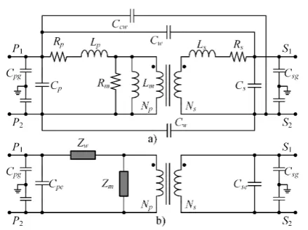
There is a significant number of medium-frequency models for power transformers, suitable for both transient simulations and steady-state operation in a large frequency range. All of these frequency-dependent models are accurate enough for the purpose of this analysis. According to [16], the model based on the classical 50-Hz, T-circuit, for single-phase, two-and three-winding transformers, shown in Fig. 1a), is appropriate to model the inductive and capacitive interaction among the coils. In the model, Rp and Rs

represent the wire resistance, mainly due to the skin effect; Lp and Ls are the leakage inductance of the

primary and secondary, respectively, both dependent on the frequency. The magnetizing impedance is modelled

Figure 1. Medium-frequency transformer model: a) lumped parameters, and b) decoupled equivalent circuit.

using a resistance, Rm, with an inductance in parallel, Lm; also the magnetizing impedance changes with

the frequency and the current level. In the proposed model, the considered capacitances, presented in Fig. 1, have the significance as follows: global turn-to-turn capacitance of the primary and secondary windings:

Cp and Cs; cross capacitance between primary and

secondary windings (divided in two capacitances):Cw;

capacitance between the input of the primary winding and the output of the secondary:Ccw; and capacitances

between the windings terminals and the ground: Cpg

andCsg.

In the decoupled model, Fig. 1b), the series impedance, Zw, includes the equivalent series

resis-tance (current dependent losses) and the equivalent leakage inductance (self and mutual leakage flux) of the two windings, in combination with part of the winding-winding capacitances. Also,Cpe (Cse) is the equivalent

capacitances ofCp (Cs) in parallel with the equivalent

cross-capacitances reflected in primary (secondary) – Miller theorem. This apparently simple model is a complex one because all of the resistors and inductors of the model are nonlinear functions of either frequency or magnetization level, or both. The capacitors also exhibit minor nonlinearities, but they are further complicated by a rough approximation to the multiple inter-winding capacitance effects that really exist in the transformer.

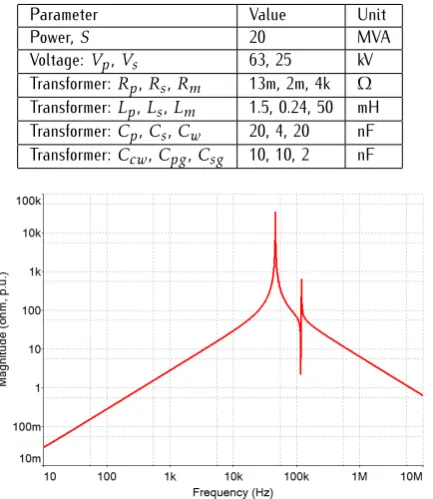
Table 1. Transformer parameters (in p.u.) used in Fig.2.

Parameter Value Unit

Power,S 20 MVA

Voltage:Vp,Vs 63, 25 kV

Transformer:Rp,Rs,Rm 13m, 2m, 4k Ω

Transformer:Lp,Ls,Lm 1.5, 0.24, 50 mH

Transformer:C_p,C_s,C_w 20, 4, 20 nF Transformer:C_cw,C_pg,C_sg 10, 10, 2 nF

Figure 2. Equivalent impedance seen by the traction side of a typical 20 MVA traction transformer.

For illustration, frequency dependence was not con-sidered and the equivalent grid impedance connected to the primary is based on 400 MVA.

However, simulation and measurement results have shown that this model is accurate enough to describe the frequency dependent behaviour of the transformer up to 30 MHz.

3. Catenary Interface

The catenary interface using pulse-width modulated converters with nearly unity power factor is the most widely used solution in modern locomotives (e.g., electric multiple unit locomotives). These converters easily provide bidirectional power flow, are modular and have a reduced harmonic content at the AC output. However, the analysis of the harmonic/resonance problem continues to be very important due to the wide range of frequencies of the injected voltages/currents.

3.1. Impedance Estimation

Several studies analyse the parallel and series reso-nances of the equivalent impedance at the traction system pantograph terminals, [8], [9], [15], [17], [18], [19], [20]. Knowledge of the harmonic impedance of catenary line is important for designing effective har-monic resonance mitigation measures. This knowledge is used in the design of harmonic filters inside the vehi-cles, the verification of harmonic limit requirements

and the prediction of system resonance, [10], [18]. The frequency response of the catenary impedance can be, in some way, calculated using similar methods to those used in the estimation of the common electric grid impedance.

A number of impedance measurement methods have been developed for this purpose: on-line and off -line methods, invasive or non-invasive, [21]. Although invasive methods give more accurate results (they achieve higher signal to noise ratio), in the context of catenary impedance estimation only on-line non-invasive methods should be considered. Nevertheless, the switching operation of PWM converters can also be considered an invasive method and thus a larger set of methods can be selected to estimate the catenary equivalent impedance.

The complex impedance, in a specified range of fre-quencies, could be obtained by direct measurement of voltages and currents; frequency domain measurements constitute a direct means of measuring the frequency characteristics of system components. The measured voltages and currents can be used to calculate the equiv-alent impedance of the catenary and the connected converters at any frequency. However, the measurement of this impedance function has proved inaccurate at those specific frequencies where parallel resonances occur. Here, the pantograph current reduces to very small values, owing to the high impedance of the line, [17]. The method is also affected by non-linearities, saturation and noise. Alternatively, spectral analysis of time domain data of system operation can be used to determine the frequency domain characteristics, [22].

A second frequency method employs correlation power spectral density (PSD) analysis on the time domain voltage and current waveforms to obtain a transfer function. This function approximates the catenary impedance as a function of frequency and a coherence coefficient is used to give a confidence level of the frequency response. The power spectral density describes the contribution of each frequency to the energy of the signal and the correlational analysis reduces the effect of noise and accounts for coupling between different frequencies due to non-linearities, [22]. In the identification of a catenary impedance model, the presence of an intermediate filter between the catenary and the on-board converters can be used in order to employ the same PSD approach, [17].

3.2. Electrical Interface

In terms of power electronics based solutions, different approaches have been employed in the past to reduce the harmonic distortion of the current injected into the catenary and thus avoiding major resonances, [6], [7], [27], [28]. The main ones are the following:

• Tuned harmonic filters, inserted between the pantograph and the high-voltage winding of the input transformer;

• Three-level converters instead of two-level con-verters on the catenary interface;

• Adaptive pulse-width modulation for the feeding power converters;

• Installation of active filters or power quality conditioners.

None of the solutions is completely effective but the use of the architecture and control flexibility of the interleaved two-level converters and three-level converters provides one the best starting approaches to deal with the issue, [7], [28], [29]. Additionally, the modularity of these two types of converters, namely the two-level ones, allows for a smooth degradation of operation in case of some types of failures, [26]. This paper focuses its attention on the two-level converters in a full-bridge topology. Thus, in order to optimize the performance of the converter sets in relation to their control, to the interaction with other converters, and their performance in the supply system, it is important to determine the catenary impedance during the converter operation.

3.3. Catenary Model

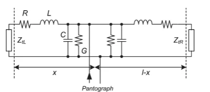
The harmonic currents and voltages occurring along the catenary give rise to travelling waves of various frequencies, which are partly reflected at the electrical line discontinuities caused by the presence of substa-tions, [3]. The most common calculation method of the impedance seen by the pantograph consists in the replacement of a many wire catenary with a two wire transmission line, which is described by the well-known transmission line equations. Considering the simplified model in Fig. 3, the impedance of the left-side line section of lengthx,ZL, is given by (1), [6], [8], [30]:

ZL=Z0

ZtLcosh(γx) +Z0sinh(γx)

Z0cosh(γx) +ZtLsinh(γx)

(1)

In Fig. 3, R, L, G and C correspond to series resistance and inductance, and parallel conductance and capacitance per unit length, respectively; ZtL and ZtRare the equivalent impedances of the left and right

line section terminations, respectively. In (1), Z0, γ andλdefine the characteristic impedance, propagation

Figure 3. Simplified model of the impedance seen by the train pantograph.

Figure 4. Contribution of each converter voltage, vci, to the

pantograph harmonic voltages.

constant, and wave speed, respectively. They are given by:

Z0=

s

R+jωL

G+jωC (2)

γ=p(R+jωL) (G+jωC) (3)

λ=√1

LC (4)

The impedance of the right-side line section is obtained by substituting l−_{x for x in (1). In this set} of parameters, the resistance R and the inductance L

are frequency-dependent due to the skin effect in the soil underneath the railway track, while the capacitance

C can be considered constant and eventually the conductance G can be neglected. The pantograph impedance is determined by the parallel of the two impedances: left and right sections, or

ZP =ZL//ZR (5)

In Fig. 4 is represented a simplified model of the contribution of one interleaved converter to the pantograph voltage.

Using the equivalent circuit in Fig. 4, the kth

harmonic voltage at the pantograph can be expressed in phasor notation as

Vsk = NT

X

i=1

Vcik Zpk

Zpk+Zsk =Vck Zpk

Table 2. Typical parameters values of railway networks.

One track Two tracks R, [Ω/km] 0.1 ... 0.3 0.07 ... 0.1 L, [mH/km] 1.2 ... 1.5 0.75 ... 0.91 G, [µS/km] 0.8 ... 1.0 1.4 ... 1.8 C, [nF/km] 11 ... 14 18 ... 20

where

Xpk=

ZinkZeqk Zink+Zeqk

(7)

and Vsk is the kth harmonic root-mean-square (RMS)

value of the pantograph voltage vs, Vcik is the kth

harmonic RMS value of the AC pulse voltage vci, and Vckis thekthharmonic RMS value of the composite AC

pulse voltage vc of the total converters. Zsk is the kth

harmonic impedance of the leakage inductance and the internal resistance of the transformer,Zink is the input

impedance seen from the pantograph, which can be quite difficult to estimate, as (1) and (5) clearly indicate. If the connection to the catenary includes some kind of filters the expression for the harmonic voltages Vsk

becomes even more complex.

The resonant frequencies depend on the position of the vehicle, the substation impedance, the type of feeding supply, etc, and are usually encountered between a few hundred Hz and several kHz, and above, depending on the circuit parameters. These frequencies are characterized by different damping coefficients which depend on:

• the respective line distance, and

• the values of the electrical line parameters at the corresponding frequency.

Typical parameters values of railway networks are presented in Table2, [3], [12], [13], [20].

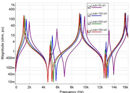
As an example, Fig. 5 shows the magnitude-frequency responses of the catenary impedance, estimated at different points, using R=0.21 Ω/km,

L=1.2 mH/km, G=0, C=11 nF/km Lsub=2 mH, and

an open end at the other side; parallel and series resonances are clearly exposed. The same parameters were used to evaluate the dependency of the catenary resonances according to the substation impedance and the results are shown in Fig.6.

The low-frequency resonances are mainly affected by this uncertainty on the catenary and substation electrical parameters and, in order to assure a reliable operation, the relevant frequency ranges should be known.

The harmonic excitation of the resonances is then suppressed if the specific frequencies, at which line resonances occur, are eliminated from the PWM

Figure 5. Magnitude (in ohm, pu) of the impedance seen by the pantograph terminals as a function of the frequency and the distance of the train from the substation, with a section length of 30 km.

Figure 6. Magnitude of the impedance seen by the pantograph terminals as a function of the substation impedance (in ohm, pu) with the train in the middle of a section with a length of 30 km.

frequency spectrum. Of great importance is also the fact that in some frequency ranges the input admittance of the vehicle can exceed some critical negative real value so that the control may become unstable, [12], [13], [31], [32].

4. Double-side Feeding Supply

interface to the transmission or distribution three-phase grid is also made using a static converter, the railway load is seen from the grid as a balanced one and with a power factor near one. So, the unbalance problem does not exist and an optimal operation of the ETS is possible. When two or more feeding points supply a power section, it implies reduced loads for each one for a specific traffic and lower catenary losses. Consequently, it allows a traction system to be fed not only from high voltage grids but also from medium voltage ones, thus reducing installation costs.

In AC railways using transformer-based substations, phase-separation sections are used mainly due to two types of reasons. The large single-phase and unbalanced railway loads originate unbalanced voltages in the transmission or distribution three-phase grids and there are standard limits for the unbalance. Then, the railway loads are connected to alternating phase pairs in the public grid in order to create a long-term kind of balance, acceptable by the relevant norms. Since the phases sequentially feeding the railway power supply system are changed, the different sections cannot be connected because of the phase difference.

The double-side feeding is not common in 50/60 Hz transformer based supply schemes but it can be envisaged in some restricted conditions or when the use of Flexible AC Transmission Systems (FACTS) devices is a possibility. For example, a Static Synchronous Compensator (STATCOM) connected in parallel with a substation can almost eliminate the three-phase current unbalance. Consequently, the voltage unbalance in the three-phase grid is also minimized, creating the conditions to connect the transformer (single-phase, V/V, Scott, etc) to an arbitrary arrangement of phases. Eventually, the no-load voltage in adjacent substations will not be exactly the same but it depends on specific conditions. If such a connection is made it will change the equivalent impedance seen by the pantograph, since it changes the section length and the impedance termination of the catenary in one side (see Fig.3).

Using the same parameters as in Fig. 6, but now considering a double-feeding scheme where the additional substation is located 65 km away from the first one, Fig.7shows the comparison of the equivalent impedance at the pantograph terminals in single and double-side feeding conditions with the train at 25 km from the first substation.

The influence of the presence of the second substation is clear: it almost does not change the first resonant frequency but the other resonant frequencies appear much closer to the first one when comparing to the single-side feeding topology. Thus, in any feeding supply scheme, an appropriate control strategy for the PWM converter(s) must be based on a prior identification of the harmonic conditions in the

Figure 7. Equivalent impedance at the pantograph terminals in single- and double-feeding supply schemes.

Figure 8. Four isolated single-phase windings supplying 4-quadrant converters operating in interleaved mode and main control requirements of each converter.

overhead supply system or on a real-time knowledge of the same conditions.

5. Interleaved PWM Converters

The three-level four-quadrant converter is one of the best choices to supply the internal DC-link from the AC catenary, [6], [7], [28]. The presence of more than one converter is required to guarantee a high redundancy in case of failure and gives the opportunity to interleave them in order to reduce the harmonic content of the absorbed current, as represented in Fig.8, [3], [6], [7], [26], [29], [33].

5.1. Interleaving Methods

The conventional (symmetric) interleaving method implies the carrier phase shift to be 1/N of a carrier cycle (with frequencyFs) whenN half-bridges

Figure 9. Single-phase full-bridge interleaving with four bridges: a) symmetric; b) regular asymmetric and c) irregular asymmetric.

that symmetric interleaving cancels all odd-order harmonics (voltage and current) of the carrier and all their sideband components, only remaining harmonics starting at sidebands of 2N Fs.

However, several objectives other than the AC ripple current can be considered, e.g. the ripple current in the common DC-bus or the frequency range where the remaining harmonics will occur. The modulation index value has also an effect in the ripple current in DC and AC branches. However, in grid-connected converters, the modulation index does not vary too much; its variation is larger when the converter is dedicated to control large amounts of reactive power (e.g. active filters) and is quite small in this application.

There are other applications where it is desirable to selectively reduce certain carrier harmonics and their sideband components. For example, the size of an Electro-Magnetic Interference (EMI) filter is usually determined by the attenuation required at a particular frequency, or range of frequencies, and will not be affected by symmetric interleaving if it does not cancel the harmonics at those frequencies. This can be achieved using a different approach to interleaving, in which the carrier phase shift is not confined to 1/(2N) of a carrier cycle and can vary from one pair of converters to another, [34]. In Fig.9 is illustrated the concept of interleaving for single-phase full-bridge inverters along with two variants: regular asymmetric interleaving and irregular asymmetric interleaving.

In regular asymmetric interleaving, the phase shifts between adjacent converters are still equal, but not equal to 1/(2N) of the carrier cycle (∆T2 in the figure). The carrier initial phase angle of thekth converter can be written as

θk= (k−1)∆θ+θ1, k= 1,2, ..., N , (8)

where ∆θ is a constant; ∆θ=π/N for symmetric interleaving. In irregular asymmetric interleaving, the carrier phase shifts are not equal and do not necessarily add to one half of a carrier period (∆T3and∆T4in the figure). Although it can be achieved almost the same minimization of THD with different phase shifts, [34], in order to obtain a large and continuous frequency range with complete harmonic elimination it should be used the symmetric interleaving method.

Interleaving is achieved by phase shifting the carrier waveforms; for N converters the carrier shift will be π/N. The four-quadrant converter constitutes a voltage source that generates higher-order line voltage harmonics. The levels and frequencies of these harmonics depend on several factors, [28], [32]:

• The switching frequency,Fs, per converter phase

leg;

• The number of interleaved bridges; the operation point of the bridge (actual voltage and power);

• The power unbalance between independent systems, i.e., for each bridge;

• The modulation strategy in the converter control.

In general ideal conditions, as stated above, the first main burst of harmonics are located as side-bands to the resultant frequency:

Fres= 2N Fs (9)

It can be easily demonstrated that perfect harmonic cancellation will only occur if all the interleaved PWM converters are operating under ideal symmetrical conditions. This means that the following conditions must be simultaneously fulfilled:

• The converter bridges parameters are perfectly balanced;

• The interleaved PWM converter bridges have equal load sharing;

• The phase shift angle of the PWM converters is symmetrical.

Figure 10. Hierarchical control of the four-quadrant converters. vdc

∗

is the reference voltage for the common DC-bus;ici

∗

is the total reference current for converteri;δi is the PWM phase for

converteri;QT

∗

is the reactive power reference.

The control system requires several current and volt-age sensors and, as a consequence, wrong or degraded measurements due to sensor or communication failures, seriously perturb the performance of the converter and may cause system malfunction. In the specific config-uration and operation mode of two or more converters some additional common blocks are required: a current sharing module in order to equalize the power in each converter, and a phase synchronization block for opti-mizing the current frequency spectrum in the primary side of the transformer, as shown in Fig.10.

Thus, a global control strategy for all PWM converters that eliminates the specific frequency bands from the harmonic spectrum of the pantograph voltage should be devised. Its main objective is avoiding the excitation of harmonic resonances under the actual operating conditions (e.g., the supply circuit equivalent impedance, the specific electrical parameters of the train, etc). It involves the real-time identification of the resonance conditions (impedance), the estimation of the state of excitation of each actual resonant frequency and the generation of an appropriate switching strategy for the converters control. As more converters operate in interleaving mode and in balanced conditions, the equivalent harmonic voltages generated in the primary side of the transformer have lower magnitudes, higher frequencies and a wider frequency spectrum. Thus, it is more difficult to excite resonances.

5.2. Proposed Method

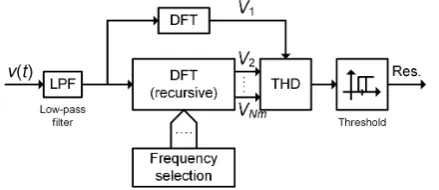
The method proposed to avoid resonant conditions is based on the detection of the catenary resonant voltage made using the discrete Fourier transform (DFT) analysis. In particular, the recursive implementation of the DFT algorithm allows fast calculations and gives the possibility of selecting the harmonics of interest.

Figure 11. Resonance detection using the recursive DFT and harmonics selection.

If the voltage signal, v(t), is sampled at a rateNsF1, where Ns is the number of samples per fundamental

period and F1 is the nominal frequency, it produces a time sequence {_vn} _{which contains Ns data points} during time interval T. The time interval, T = 1/F1, is the time window for calculating the DFT. The DFT producing the mth harmonic of {_vn} _{at the frequency}

mF1, and at instantk, can then be written as:

Vm(k) = k

X

n=k−_Ns+1

vnexp(−j2π(n−1)m/Ns) (10)

Writing the same expression for instant k−_{1 and} subtracting the two, it is obtained the recursive version of the DFT for harmonic orderm:

Vm(k) =Vm(k−1) + [vk−vk−_Ns] exp(−j2π(k−1)m/N_s) (11) The recursive expression for the DFT of{_vn}_{is based} on the history of the DFT and the difference betweenkth

and (k−_Ns)th_{values in the time sequence.}

The DFT analysis of the primary voltage selects the frequency range where resonance is most likely to occur. In the present study, this range is located between 1000 Hz and 2000 Hz and is dependent on the catenary and substation electrical parameters, as pointed out in Section 3. Aggregation of the harmonic voltages in this range, using the total harmonic distortion (THD) parameter, gives a measure of the resonance conditions:

T HD(%) = 100 1

V1

v u t_Nm

X

m=2

Vm2 (12)

If the THD is above a specified level/threshold, it is classified as resonance, as depicted in Fig. 11. A hysteresis window must be included in order to achieve a proper return to normal conditions.

Table 3. Parameters values used in the simulations.

Parameter Value/Type

Substation nominal power,S 20 MVA Substation impedance,Z_sub 0.003+i0.02 p.u. Transformer voltage: pr./sec. 25 kV/0.9 kV Transformer impedance 0.01+i0.02 p.u. DC-bus voltage,v_dc 1.4 p.u. Nominal frequency,F1 50 Hz

Switching frequency,Fs 600 Hz

AC current controller dq-axes, PI-type

normal value and there is no PWM synchronization between any converter. This operation mode is a degraded one since the switching losses are increased and the catenary current is more distorted but the resonance condition is avoided.

6. Simulation Results

A catenary with a length of 30 km divided into 6 sections was used with the parametersR=0.21 Ω/km,

L=1.2 mH/km,G=0,C=11 nF/kmLsub=2 mH, and an

open end at the other side. With these parameters the first resonant frequency is located between 1380 and 1400 Hz along the all catenary, as can be concluded from Fig.5. The other relevant parameters used in the simulations are listed in Table3.

In order to achieve decoupled power control, a vector control approach was used for the AC current controller using the 90º phase delay for creating the beta component of the current, [35].

The two relevant conditions related to the four-quadrant converters are exemplified in the next figures, where the train position is located 10 km away from the open end. Fig.12shows two secondary currents and the primary current (converter 1, which serves as phase reference, and converter 3, with a 90º shifted PWM carrier; converters 2 and 4 have carriers phase shifted by 45º and 135º, respectively) while Fig. 13 contains the frequency spectrum of one secondary current and of the primary current. It is clearly demonstrated the harmonic cancellation occurring in the primary current.

6.1. Unbalanced Current

As referred before, two conditions negatively affect the harmonic cancellation in the primary current and thus the avoidance of resonances can be no longer possible: current unbalance and phase shift asymmetry. Fig.14shows the result of a malfunction in the current balancing module: at t=0.25 s, converter 1 and 2 become not balanced (withIs1=1.3 p.u. andIs2=0.7 p.u.) while converters 3 and 4 are still balanced; also shown is the primary current.

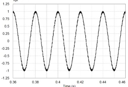
The steady-state catenary voltage is shown in Fig. 15 and its harmonic spectrum in Fig. 16; in the two

Figure 12. Two secondary currents and the primary current in normal operation mode. Traces: Is1 - AC current of converter 1, Is3 - AC current of converter 3, Ip - primary current.

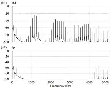
Figure 13. Secondary and primary currents frequency spectrum showing harmonic cancellation. Traces: Is1 - AC current of converter 1, Ip - primary current.

figures, and due to the presence of harmonics in the primary current centred at 1.2 kHz (twice the switching frequency) and multiples, a small excitation of the resonance mode can be noticed.

The steady-state primary (catenary) voltage is shown in Fig. 15 and its harmonic spectrum in Fig. 16; in the two figures, and due to the non-cancellation of harmonics in the primary current, components centred at multiples of 1.2 kHz (twice the switching frequency) have relevant magnitudes and a relatively small excitation of the resonance mode is present (at around 1400 Hz, as referred above).

6.2. Loss of Synchronization

Figure 14. Transient and steady-state current unbalance in converters 1 and 2. Traces: Is1 AC current of converter 1, Is2 -AC current of converter 2, Ip - primary current.

Figure 15. Steady-state primary (catenary) voltage (Vpr) under current unbalance in the different converters.

Figure 16. Frequency spectrum of the primary voltage (Vpr) showing components around twice the switching frequency.

Figure 17. Synchronization loss between converters 1 and 2, starting att=0.3 s. Traces: Is1 - AC current of converter 1, Is2 - AC current of converter 2, Ip - primary current.

Figure 18. Steady-state primary voltage (Vpr) near resonance conditions originated by loss of synchronization.

the fulfilment of this condition. Fig.17shows the result of a loss of synchronization (starting att=0.3 s) between converters 1 and 2: converter 1 and 2 have in-phase PWM signals while converters 3 and 4 still have the correct phase shift. As can be seen, currents Is1 and Is2 are in phase and the primary current is more distorted. The steady-state catenary voltage is shown in Fig.18 and its harmonic spectrum in Fig.19. In the two figures, and due to the non-cancellation of harmonics in the primary current, components centred at multiples of 1.2 kHz (twice the switching frequency) have relevant magnitudes. Thus, a substantial excitation of the first resonance mode is present (at around 1400 Hz, as referred above).

6.3. Control Reconfiguration

Figure 19. Frequency spectrum of the primary voltage (Vpr), showing resonance conditions.

Figure 20. Primary voltage resonance detection and avoidance in single-side feeding (resonance startst=0.31 s and is detected at aroundt=0.33 s). Traces: Vpr - primary voltage, THD - total harmonic distortion, L_sync - loss of synchronism, F_sync - fault of synchronism.

from the substation. Additional parameters are those in Table3.

In Fig. 20, is given an example of the resonance detection according to the proposed principle. At

t=0.31 s the converters start to operate out of synchronism (signal L−sync) and this condition is present until t=0.39 s. The loss of synchronization between converters starts the occurrence of resonance conditions with an increase in THD, as can be seen in the primary voltage. After a delay of around one cycle (when THD>10%) the method detects this condition (signal F−sync is activated) and changes the switching frequency accordingly. As can be seen the primary voltage, Vpr, rapidly returns to a non-resonant condition and, if the synchronism operation returns, the converters also return to its original switching frequency.

Figure 21. One secondary current and the primary current in normal operation (t <0.31 s and t >0.39 s), and when a resonance condition is detected. Traces: Is1 - AC current of converter 1, Ip - primary current.

Figure 22. Steady-state primary voltage (Vpr) during loss of synchronism with different switching conditions.

In Fig.21 is shown one secondary current (Is1) and the primary current (Ip) for the same conditions as in Fig. 20. After the resonance detection, the switching frequency is changed to twice the nominal one in all converters without any type of synchronization. As can be seen, during loss of synchronism the converter current (Is1) becomes more sinusoidal but the primary current increases its distortion. This due to the non-cancellation of harmonics in the primary current as the converters are not operating in interleaving mode.

On the other hand, as shown in Fig. 22 in steady-state operation, the catenary voltage slightly increases its distortion when operating in this degraded mode but only in a small magnitude, as quantified in Fig.23.

Figure 23. Frequency spectrum of the primary voltage (Vpr) with different switching conditions.

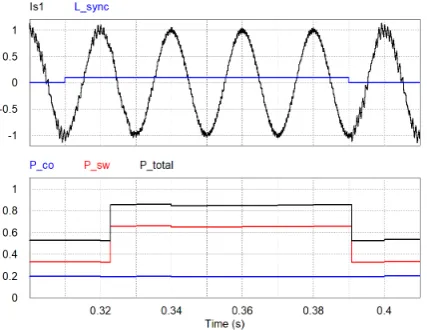
Figure 24. Conduction and switching losses in normal and degraded conditions (resonance starts att=0.31 s). Traces: Is1 AC current of converter 1, L_sync loss of synchronism, P_co -conduction losses, P_sw - switching losses, P_total - total losses.

As referred before, the detection of a resonance condition changes the converter switching frequency, duplicating it in the use case. This increase affects the converter losses. Converter losses have mainly two components: conduction losses and switching losses. Conduction losses do not depend on the switching frequency; switching losses are mainly a linear function of the switching frequency and both are proportional to the DC-bus voltage level and the AC current. It is shown in Fig.24the evolution of the losses in converter 1 (conduction, switching and total losses) for the same conditions present in Fig. 20 and Fig. 21. In normal operation, the conduction losses account for near 20% of the maximum converter losses and switching losses are around 33%. When a resonance condition is detected (at t=0.323 s) the switching frequency increases (the converter current is less distorted) and the switching losses duplicate thus resulting in a global increase of the converter total losses.

Figure 25. Primary voltage resonance detection and avoidance in double-side feeding (resonance starts at t=0.31 s). Traces: Vpr - primary voltage, THD - total harmonic distortion, L_sync - loss of synchronism, F_sync - fault of synchronism.

A second scenario is considered and refers to the double-side feeding supply architecture, as briefly described in Section 4. In this condition, catenary voltage resonance can occur in slightly different frequency ranges since supply sections are longer and an additional substation is present. It were considered the same catenary and substation parameters as used before with the train located at 40 km from the first substation. In Fig. 25 the conditions applied are: between t=0.31 s and t=0.39 s the converters start to operate out of synchronism. After a detection delay (when THD>10%) the method detects this condition and changes the switching frequency accordingly. As before, the primary voltage rapidly returns to a non-resonant condition and, if the synchronism operation returns, the converters also return to its original switching frequency.

As mentioned before, double-side feeding presents different resonance conditions and this can be observed either in the steady-state voltage waveform (before

t=0.31 s) and in the magnitude of the resonance voltage before detection. It is worth mentioning that the steady-state voltage ripple with a higher switching frequency is smaller; it is the opposite in relation to the single-side feeding condition. For the currents, the conclusion is the same as the one obtained from Fig.21: with a higher switching frequency each converter current becomes less distorted but the non-symmetrical interleaved operation produces a more distorted primary current.

Figure 26. Resonance caused by changing from traction to regeneration mode, starting at t=0.2 s, in single-side feeding scheme. Traces: Vpr - primary voltage, Ip - primary current, Id1_r - reference value for the active current component of converter 1, THD - total harmonic distortion, L_sync - loss of synchronism, F_sync - fault of synchronism.

behaviour of the catenary voltage and primary current (Vpr and Ip, respectively) when the motoring mode changes from full traction to full braking, at t=0.2 s. As the converter control is based in vector control, the inversion of Id1_r (reference value for the active current component of Converter 1, at a rate of 100 p.u./s) represents the power inversion mode. With the loss of synchronism, the voltage resonance starts, is detected as in the previous tests and the same counter measures are applied. After a small transient, the resonance condition is eliminated and the regenerative mode (primary voltage and current in phase opposition with power factor approximately equal to one) runs smoothly. The result applies to the single-side feeding architecture but a similar behaviour occurs in a double-side supply structure.

The presented approach requires the detection of the resonance occurrence, e.g. using a total harmonic distortion measurement, and knowledge of the equivalent characteristic impedance seen by the pantograph terminal in order to change the switching frequency. That impedance is mainly dependent on the catenary and return circuit distributed parameters and substation impedance and not on the train position or the number of trains in the track, as shown in Fig.6and also demonstrated in [6], [8], [11]. Therefore, it could be a viable solution to increase the robustness of the interface between the fixed installations of the electrical system and the moving trains.

7. Conclusions

Modern electric traction systems employ four-quadrant converters operating in parallel with an interleaved

switching strategy in order to achieve a very low current harmonic distortion. However, the existence of power unbalance between the converters or the loss of synchronism between the converters controllers originates resonance effects in the overhead contact line that can create high levels of harmonic voltages along the catenary.

This paper presented a control reconfiguration approach capable of maintaining the converters oper-ating in parallel without exciting relevant resonances, either in the conventional single-side feeding architec-ture and in a possible double-side feeding arrangement.

Acknowledgements. The research has received funding from

the FCT (Fundação para a Ciência e Tecnologia) under grant PD/BD/128051/2016. This work was partially supported by: FCT R&D Unit SYSTEC - POCI-01-0145-FEDER-006933/SYSTEC funded by FEDER funds through COMPETE 2020 and by national funds through the FCT/MCTES, and co-funded by FEDER, in the scope of the PT2020 Partnership Agreement.

References

[1] Shift2Rail(2014) Shift2Rail Multi-Annual Action Plan.

Brussels.

[2] International Energy Agency(2019)The Future of Rail.

Opportunities for energy and the environment. Paris. [3] Brenna, M., Foiadelli, F. and Zaninelli, D. (2018)

Electrical Railway Transportation Systems. (IEEE Press -Wiley), 1st ed., Hoboken, New Jersey.

[4] Kneschke, T.A. (1985) Control of utility system

unbalance caused by single-phase electric traction.IEEE Tr. on Industry Applications,21(6): 1559–1570.

[5] Chen, B.-K.andGuo, B.-S.(1996) Three phase models

of specially connected transformers.IEEE Tr. on Power Delivery,11(1): 323–330.

[6] Holtz, J. and Klein, H.-J. (1989) The propagation of

harmonic currents generated by inverter-fed locomotives in the distributed overhead supply system.IEEE Tr. on Power Electronics,4(2): 168–174.

[7] Chang, G.W., Lin, H.-W. and Chen, S.-K. (2004)

Modeling characteristics of harmonic currents generated by high-speed railway traction drive converters.IEEE Tr. on Power Delivery,19(2): 766–773.

[8] Zynovchenko, A., Xie, J.,Jank, S.andKlier, F. (2005)

Resonance phenomena and propagation of frequency converter harmonics in the catenary of railways with single-phase A.C. In Proc. of the EPE 2005, 11-14 September, Dresden, Germany.

[9] Wang, B., Han, X.D., Gao, S.B., Huang, W. and Jiang, X.F.(2013) Harmonic power flow calculation for

high-speed railway traction power supply system. InJia L. et al. (eds.), Proc. of the 2013 Int. Conf. on Electrical and Information Technologies for Rail Transportation (EITRT 2013), vol. I, 11–26.

[10] Hu, H., He, Z.andGao, S.(2015) Passive filter design

[11] Janssen, M.P., Gonçalves, P.G., Santo, R.P. and Smulders, H.M.(2008) Simulations and measurements

on electrical resonances on the Portuguese 25 kV network. InProc. of the 8th World Congress on Railway Research, WCRR 2008, May 18-22, Seoul, South Korea. [12] Suarez, J. (2014) Étude et modélisation des intéractions

éléctriques entre les engins et les installations fixes de traction éléctrique 25 kV-50 Hz.PhD thesis, GEET-INP, Toulouse, France.

[13] Hu, H., Tao, H., Blaabjerg, F., Wang, X., He, Z. and Gao, S.(2018) Train-network interactions and stability

evaluation in high-speed railways - Part I: phenomena and modeling. IEEE Tr. on Power Electronics, 33 (6): 4627–4642.

[14] Lee, H., Lee, C., Jang, G. and Kwon, S.-H. (2006)

Harmonic analysis of the Korean high-speed railway using the eight-port representation model. IEEE Tr. on Power Delivery,21(2): 979–986.

[15] Brenna, M., Capasso, A., Falvo, M.C., Foiadelli, F., Lamedica, R. and Zaninelli, D. (2011) Investigation

of resonance phenomena in high speed railway supply systems: Theoretical and experimental analysis.Electric Power Systems Research,81: 1915–1923.

[16] Chimklai, S.andMarti, J.(1995) Simplified three-phase

transformer model for electromagnetic transient studies. IEEE Tr. on Power Delivery,10(3): 1316–1325.

[17] Holtz, J.andKrah, J.O.(1990) On-line identification of

the resonance conditions in the overhead supply line of electric railways.Electrical Engineering,74(1): 99–106. [18] Mariscotti, A. and Pozzobon, P. (2003) Synthesis of

line impedance expressions for railway traction systems. IEEE Tr. on Vehicular Technology,52(2): 420–430. [19] Dolara, A., Gualdoni, M.andLeva, S. (2012) Impact

of high-voltage primary supply lines in the 2x25 kV-50 Hz railway system on the equivalent impedance at pantograph terminals.IEEE Tr. on Power Delivery,27(1): 164–175.

[20] Monjo, L. andSainz, L.(2015) Study of resonances in

1x25 kV AC traction systems.Electric Power Components and Systems,43(15): 1771–1780.

[21] Robert, A.andDeflandre, T.(1997) Guide for assessing

the network harmonic impedance. In Proc. of the 14th Int. Conf. and Exhibition on Electricity and Distribution, CIRED 1997, (IEE Conf. Publ. No. 438), 2-5 June, Birmingham, UK.

[22] Girgis, A.andMcManis, R.B.(1989) Frequency domain

techniques for modelling distribution or transmission networks using capacitor switching induced transients. IEEE Tr. on Power Delivery,4(3): 1882–1890.

[23] Hoffmann, N.andFuchs, F.W.(2014) Minimal invasive

equivalent grid impedance estimation in inductive-resistive power networks using extended Kalman filter.

IEEE Tr. on Power Electronics,29(2): 164–175.

[24] Duda, K., Borkowski, D.andBień, A. (2009)

Compu-tation of the network harmonic impedance with chirp z-transform.Metrology and Measurement Systems,16(2): 299–312.

[25] Xu, W., Huang, Z., Cui, Y. and Wang, H. (2005)

Harmonic resonance mode analysis.IEEE Tr. on Power Delivery,20(2): 1182–1190.

[26] Perreault, D.J.andKassakian, J.G.(1997) Distributed

interleaving of paralleled power converters. IEEE Tr. on Circuits and Systems – I: Fundamental Theory and Applications,44(8): 728–735.

[27] Tan, P.-C.,Loh, P.C.andHolmes, D.G.(2005) Optimal

impedance termination of 25-kV electrified railway systems for improved power quality.IEEE Tr. on Power Delivery,20(2): 1703–1710.

[28] Zhang, R.,Lin, F.,Yang, Z.,Cao, H.andLiu, Y.(2017)

A harmonic resonance suppression strategy for a high-speed railway traction power supply system with a SHE-PWM four-quadrant converter based on active-set secondary optimization.Energies,10, 1567–1589. [29] Holtz, J. and Krah, J.O. (1992) Suppression of

time-varying resonances in the power supply line of AC locomotives by inverter control. IEEE Tr. on Industrial Electronics,39(3): 223–229.

[30] Qiujiang, L., Mingli, W., Junki, Z., Kejian, S. and Liran, W. (2018) Resonant frequency identification

based on harmonic injection measuring method for traction power supply systems.IET Power Electronics,11

(3): 585–592.

[31] Sun, J. (2011) Impedance-based stability criterion for

grid-connected inverters. IEEE Tr. on Power Electronics,

26(11): 3075–3078.

[32] Cespedes, M.andSun, J.(2014) Adaptive control of

grid-connected inverters based on online grid impedance measurements.IEEE Tr. on Sustainable Energy,5(2): 516– 523.

[33] Youssef, A.B.,El Khil, S.K. Slama-Belkhodja, I.(2013)

State observer-based sensor fault detection and isolation, and fault tolerant control of a single-phase PWM rectifier for electric railway traction.IEEE Tr. on Power Electronics,28(12): 5842–5853.

[34] Beechner, T.andSun, J.(2009) Asymmetric interleaving

- a new approach to operating parallel converters. In Proc. of the 2009 IEEE Energy Conversion Congress and Exposition, 20-24 Sept. San Jose, CA, USA, 99–105. [35] Bahrani, B. andRufer, A. (2013) Optimization-based