Nonlin. Processes Geophys., 17, 187–200, 2010 www.nonlin-processes-geophys.net/17/187/2010/ © Author(s) 2010. This work is distributed under the Creative Commons Attribution 3.0 License.
Nonlinear Processes
in Geophysics
Estimating the diffusive heat flux across a stable interface forced
by convective motions
C. Chemel1, C. Staquet2, and J.-P. Chollet2
1NCAS-Weather, Centre for Atmospheric & Instrumentation Research, University of Hertfordshire, Hatfield, UK 2Laboratoire des Ecoulements G´eophysiques et Industriels, CNRS/UJF/INPG, Grenoble, France
Received: 22 April 2009 – Revised: 16 March 2010 – Accepted: 18 March 2010 – Published: 8 April 2010
Abstract. Entrainment at the top of the convectively-driven boundary layer (CBL) is revisited using data from a high-resolution large-eddy simulation (LES). In the range of val-ues of the bulk Richardson numberRiBstudied here (about 15–25), the entrainment process is mainly driven by the scouring of the interfacial layer (IL) by convective cells. We estimate the length and time scales associated with these convective cells by computing one-dimensional wavenum-ber and frequency kinetic energy spectra. Using a Taylor assumption, based upon transport by the convective cells, we show that the frequency and wavenumber spectra follow the Kolmogorov law in the inertial range, with the multiplica-tive constant being in good agreement with previous mea-surements in the atmosphere. We next focus on the heat flux at the top of the CBL,Fi, which is parameterized in classical
closure models for the entrainment rateweat the interface. We show thatFi can be computed exactly using the method
proposed by Winters et al. (1995), from which the values of a turbulent diffusivityKacross the IL can be inferred. These values are recovered by tracking particles within the IL us-ing a Lagrangian stochastic model coupled with the LES. The relative difference between the Eulerian and Lagrangian values ofKis found to be lower than 10%. A simple expres-sion ofweas a function ofK is also proposed. Our results are finally used to assess the validity of the classical “first-order” model forwe. We find that, whenRiBis varied, the values forwe derived from the “first-order” model with the exact computation ofFi agree to better than 10% with those
computed directly from the LES (using its definition). The simple expression we propose appears to provide a reliable estimate ofwefor the largest values ofRiBonly.
Correspondence to: C. Staquet ([email protected])
1 Introduction
An interfacial layer (IL) divides the clear convective atmo-spheric boundary layer (CBL) and the stably-stratified free atmosphere (FA) above. The IL is forced by turbulent mo-tions, which are primarily triggered by ground surface heat-ing. Indeed, the main mechanism of turbulence production within the well-mixed part of the CBL (referred to as the mixed layer) is buoyant convection, with a possible wind-shear contribution. The penetration of rising thermals into the FA is associated with an entrainment of air down into the mixed layer (e.g. Sorbjan, 1996). As a result, the CBL deep-ens or equivalently the IL raises. A mixed layer with similar structure and dynamics also forms in the upper ocean when cooling occurs at the surface. As pointed out for instance by Stevens and Lenschow (2001), the modeling of the entrain-ment process is an essential issue in any attempt to parame-terize the CBL in large-scale models, for both atmospheric and oceanic applications. Indeed, only a few parameteriza-tion schemes of boundary-layer flow within meso-scale mod-els represent explicitly the entrainment process (e.g. Hong et al., 2006). The representation of the entrainment process is also an issue for air quality prediction. Mean vertical gra-dients of concentrations of atmospheric constituents are close to zero within the mixed layer. Hence, the rising rate of the mixed layer into the FA determines partly the concentrations at the ground surface (e.g. Cai and Luhar, 2002).
The entrainment process across a buoyancy interface (such as the IL) due to turbulent motions has been studied exten-sively in laboratory experiments. Hopfinger (1987) and Fer-nando (1991) gave a thorough review for an IL that is forced by grid turbulence. In grid turbulence experiments, the en-trainment process is discussed classically as a function of a bulk Richardson number at the interface,Ri=1bl0/(σu)20 (using the notation of Hannoun and List, 1988), where1b
is the buoyancy jump across the interface, andl0and(σu)20
are the integral length scale and variance of the turbulence in the absence of the interface. Entrainment and resulting mixing of entrained fluid occur roughly for 1<Ri<50.
Han-noun and List (1988) showed that for this range ofRi values,
mixing results from internal gravity wave breaking at the in-terface. Below this range, mixing occurs as if the fluid were homogeneous, and above that range, mixing occurs through pure molecular diffusion. As stressed for instance by Sulli-van et al. (1998), the extension of the results from grid turbu-lence experiments is actually debatable since the CBL con-tains large-scale organized structures, which are not present in such experiments.
The thermally-driven convection tank experiment of Dear-dorff et al. (1980) was designed to mimic the CBL dynamics. The stability of the buoyancy interface was also characterized by a bulk Richardson number at the interface, defined as
RiB=g β 12zi/w∗2, (1)
whereg is the gravitational acceleration, β the coefficient of thermal expansion, 12the potential temperature1jump across the interface,zi the mixing depth, andw∗the
convec-tive velocity (defined below). The quantitiesβ,12,zi and w∗refer to horizontally averaged quantities. The convective velocity within the mixed layer is expressed as
w∗=(g βFszi)1/3, (2)
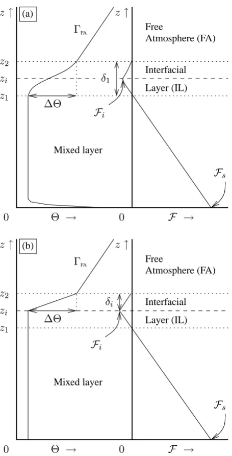
whereFs=w020sis the horizontally averaged heat flux just above the surface. Typical vertical profiles of potential tem-perature2and heat fluxF=w020 are depicted in Fig. 1a (and are further discussed in Sect. 4.4). For a broad range of RiBvalues (about 2–85), which are usually observed in the atmosphere, the entrainment rate,we=dtzi(with dt≡d/dt),
was found to vary as
we/w∗=ARiB−1, (3)
where the dimensionless parameterAis the entrainment ratio and is close to 0.25. There is actually a wide spread in the values ofAreported in the literature, though it is often found to be around 0.2 in the regime of equilibrium entrainment (i.e. when the mixed layer dynamics has reached a quasi-steady state). The parameterization ofA, and more generally ofwe, is at the heart of the debate on entrainment.
The most common parameterizations of we are the so-called “zero-order” and “first-order” jump models, which were proposed by Lilly (1968) and Betts (1974), respectively. In the “zero-order” model, the thickness of the IL is assumed infinitesimal, while the potential temperature profile exhibits a jump across that interface. In “first-order” models, the fi-nite thickness of the IL is taken into account (see for instance 12is actually the virtual potential temperature, namely the po-tential temperature modified by humidity effects. In the following, for simplicity, we shall use the denomination potential temperature for2(in place of virtual potential temperature).
Fig. 1b). In both models, the altitude of the IL is the mixing depthzi and is defined as the level where the heat fluxFi is
minimum (being negative). The main issue in these models is to derive a closure for this flux. Fedorovich et al. (2004) presents more general formulations for the entrainment law and reviewed methods for determining entrainment parame-ters from large-eddy simulation (LES) outputs.
Sullivan et al. (1998) used LESs to investigate the convec-tive entrainment process and the structure of the IL over a wide range ofRiBvalues (about 15–45). The authors showed that the finite thickness of the IL needs to be considered in an entrainment law formulation derived from a jump model. In other terms, the “zero-order” jump model was found insuf-ficient, especially at lowRiB. Conversely, the “first-order” jump model was found to work well. Fedorovich et al. (2004) also found that the “zero-order” parameterization is insuffi-cient outside the regime of equilibrium entrainment.
In this study, we present results from a high-resolution LES of the convectively-driven boundary layer initialized by a commonly used sounding of Day 33 of the Wangara ex-periment (Clarke et al., 1971). Our main purpose is to show that the heat flux at the interface (i) can be computed exactly, using the method proposed by Winters et al. (1995), and (ii) can be expressed in terms of a vertical turbulent diffusivity
K, which we also obtain from Lagrangian particle tracking. This allows us to assess the validity of the commonly used “first-order” model to parameterizeweand to provide a sim-ple expression ofwein terms ofK.
Several LES studies have been conducted to investigate the entrainment process in the CBL (see for instance Stevens and Lenschow, 2001). Sorbjan (1996) carried out LES ex-periments to analyse the effects, on entrainment, of the ver-tical potential temperature gradient in the FA, hereafter de-noted by0FA (see Fig. 1). The entrainment rate was found to depend on0FA but the entrainment ratio varied only slightly in the range 0.2–0.3 for values of0FA from 1 to 10 K km
−1 (which are usually observed in the atmosphere). In addition, the statistical moments in the lower 90% portion of the mixed layer were found almost independent of0FA. Lewellen and Lewellen (1998) also examined the convective entrainment process and stressed that the entrainment rate is controlled by the turbulent transport at the scale of the boundary layer and is relatively insensitive to the smaller scales of mixing near the IL. This confirms earlier findings by Linden (1975) (for grid-generated turbulence), Manins and Turner (1978), and Schmidt and Schumann (1989). Otte and Wyngaard (2001) focused on the properties of the IL and found that turbulence there behaves as in stably-stratified flows, consistent with the work of Hannoun and List (1988).
C. Chemel et al.: Estimating the diffusive heat flux across a stable interface forced by convective motions 189
C. Chemel et al.: Estimating the diffusive heat flux across a stable interface forced by convective motions 3
δ
1z
iz
10
z
↑
z
↑
0
z
2Θ
→
F →
F
sΓ
FA∆Θ
Interfacial Layer (IL) Free Atmosphere (FA) Mixed layerF
i (a)δ
iz
iz
10
z
↑
0
z
2Θ
→
F →
F
sΓ
FA Interfacial Layer (IL) Free Atmosphere (FA) Mixed layerz
↑
F
i (b)∆Θ
Fig. 1. (a) Typical vertical profiles of potential temperatureΘand heat fluxFfor the convectively-driven boundary layer. (b) Same as (a) for the ‘first-order’ model proposed by Betts (1974) (referred to as ‘FOM1’ in § 4.4). All parameters are defined in the text.
In § 4, we show that the heat flux at the interface can be computed exactly and that a turbulent diffusivity across the interface can be inferred, whose values are recovered from the tracking of fluid particles within the interface. These re-sults are finally used to assess the validity of the ‘first-order’ model. Conclusions are given in § 5.
2 Model description and setup
2.1 The LES model
The numerical experiments presented in this paper were conducted with the Advanced Regional Prediction System (ARPS), a non-hydrostatic, compressible LES code devoted to meso-scale and small-scale atmospheric flows. Xue et al. (2000; 2001) gave an extensive description of the model for-mulation and applications.
The basic idea of physical LES is the ‘filtering approach’ to separate the small scales from the large scales (see Lesieur and M´etais, 1996, for a review). In this approach, a low-pass spatial filter (denoted by a tildee hereafter) is applied to the turbulent fields. In the present study the characteris-tic width of the filter∆e is equal to the geometric average of the grid size in the three spatial directions. The application of this filter to the mass- and momentum-conservation equa-tions, assuming that the filtering operation commutes with differentiation, results in
∂tuei+uej∂juei = [∂j(µ ∂juei)−∂ipe]/ρe
−∂jτij+ (g−2Ω×eu)i
∂tρe+∂j(uejρe) = 0
, (4)
whereu,p, andρare the velocity, the pressure and the den-sity fields, respectively,µis the dynamic viscosity, and the subscripts (i, j) ∈ {1,2,3} refer to the geometrical coor-dinates. For convenience, we will also adopt the follow-ing notation: (x1, x2, x3) ≡ (x, y, z)and(u1, u2, u3) ≡
(u, v, w). The termsτij=ugiuj−ueiuejand−2Ω×ue, with
Ωbeing the Earth’s angular velocity, represent the subgrid-scale (SGS) turbulent stress and the Coriolis acceleration, respectively. The SGS term must be parameterized as a function of the filtered variables. For this purpose, an eddy-viscosity model is used, namely
τij−δijτkk/3 =−2νtSfij, (5)
where δij is the Kronecker delta symbol and Sfij = (∂juei+∂iuej)/2is the filtered strain-rate tensor. νt is the SGS turbulent viscosity, which is expressed as a function of the filtered variables through a mixing length formulation. This formulation yieldsνt = 0.1ℓ e1/2, wheree =τkk/2is the turbulent kinetic energy of the subgrid scales andℓ is a typical subgrid length scale, which accounts for the effects of stratification (Deardorff, 1980). For a grid size with an aspect ratio in the order of unity,ℓis equal to∆efor unstable or neu-tral cases and min(∆e,0.76√e N−1
)for stable case, where
N = (g β ∂3Θ)e 1/2
is the buoyancy frequency. Note that for a larger aspect ratio, we need to set the vertical length scale apart from the horizontal one.
The prognostic equation foreis
∂te+∂j(ueje) = 2νtSfij
2
+ (νt/Prt)N2 + 2∂j(ρ νe t∂je)/ρe−ε
, (6)
Fig. 1. (a) Typical vertical profiles of potential temperature2and heat fluxFfor the convectively-driven boundary layer. (b) Same as (a) for the “first-order” model proposed by Betts (1974) (referred to as “FOM1” in Sect. 4.4). All parameters are defined in the text.
In Sect. 4, we show that the heat flux at the interface can be computed exactly and that a turbulent diffusivity across the interface can be inferred, whose values are recovered from the tracking of fluid particles within the interface. These re-sults are finally used to assess the validity of the “first-order” model. Conclusions are given in Sect. 5.
2 Model description and setup
2.1 The LES model
The numerical experiments presented in this paper were conducted with the Advanced Regional Prediction System (ARPS), a non-hydrostatic, compressible LES code devoted to meso-scale and small-scale atmospheric flows. Xue et al. (2000; 2001) gave an extensive description of the model for-mulation and applications.
The basic idea of physical LES is the “filtering approach” to separate the small scales from the large scales (see Lesieur and M´etais, 1996, for a review). In this approach, a low-pass spatial filter (denoted by a tildeehereafter) is applied
to the turbulent fields. In the present study the characteris-tic width of the filter1eis equal to the geometric average of
the grid size in the three spatial directions. The application of this filter to the mass- and momentum-conservation equa-tions, assuming that the filtering operation commutes with differentiation, results in
∂tuei+uej∂juei =
∂j µ∂juei
−∂iep
/eρ
−∂jτij+(g−2×eu)i ∂tρe+∂j uejeρ
=0
, (4)
where u, p, and ρ are the velocity, the pressure and the density fields, respectively,µis the dynamic viscosity, and the subscripts(i,j )∈ {1,2,3}refer to the geometrical coor-dinates. For convenience, we will also adopt the following notation: (x1, x2, x3)≡(x, y, z)and(u1, u2, u3)≡(u, v, w). The termsτij=ugiuj−ueiuej and−2×eu, withbeing the
Earth’s angular velocity, represent the subgrid-scale (SGS) turbulent stress and the Coriolis acceleration, respectively. The SGS term must be parameterized as a function of the filtered variables. For this purpose, an eddy-viscosity model is used, namely
τij−δijτkk/3= −2νtSfij, (5)
where δij is the Kronecker delta symbol and Sfij = ∂juei+∂iuej
/2 is the filtered strain-rate tensor. νt is the
SGS turbulent viscosity, which is expressed as a function of the filtered variables through a mixing length formulation. This formulation yieldsνt=0.1`e1/2, wheree=τkk/2 is the
turbulent kinetic energy of the subgrid scales and`is a typ-ical subgrid length scale, which accounts for the effects of stratification (Deardorff, 1980). For a grid size with an aspect ratio in the order of unity,`is equal toe1for unstable or
neu-tral cases and min e1,0.76
√ eN−1
for stable case, where N= g β ∂32e
1/2
is the buoyancy frequency. Note that for a larger aspect ratio, we need to set the vertical length scale apart from the horizontal one.
The prognostic equation foreis ∂te+∂j ueje
=
2νtSfij
2
+(νt/Prt)N2
+2∂j eρ νt∂je
/ρe−ε
, (6)
whereε=Cεe3/2/`is the dissipation rate of turbulent kinetic
energy and the coefficientCε has the value 3.9 at the lowest
vertical level and 0.93 otherwise. The turbulent Prandtl num-ber is parameterized as Prt=1/1+ 2`/e1
, from where the SGS turbulent thermal diffusivityκt=νt/Prtcan be inferred.
The energy-conservation equation for2eis written as ∂te2+∂j uej2e
=∂j λ∂j2e
/ eρ cp−∂jϕj, (7)
whereλis the thermal conductivity, cpis the specific heat at constant pressure, andϕj=2ugj−e2uej is the SGS
turbu-lent heat flux, which is expressed as a function of the filtered potential temperature gradient∂j2e, namely
−ϕj=κt∂j2.e (8)
2.2 Model setup
The model is initialized using vertical profiles of potential temperature, horizontal wind, and vapor mixing ratio taken at 09:00 EST during Day 33 of the Wangara experiment held in Hay, Australia (Clarke et al., 1971). The wind profile is almost shear-free up to the top of the domain and the ver-tical potential temperature gradient in the FA,0FA, is about 10 K km−1. The ground surface is heated through the ab-sorption of solar radiation. This results in a diurnal variation in the ground surface temperature and turbulent heat fluxes, which trigger convective motions.
A good representation of land surface characteristics was found necessary to reproduce realistically the atmospheric boundary-layer structure and its evolution. The land-surface energy budget was calculated by a simplified soil-vegetation model (Noilhan and Planton, 1989; Pleim and Xiu, 1995). The soil type was loam and the vegetation type was desert. The roughness length was 0.24 m, the leaf area index was 0.1 and the fractional vegetation coverage was 5%. The ground surface temperature was initialized to its observed value at 09:00 EST (278.7 K). There was no direct measurement of the deep surface temperature, so that its initial value was evaluated from the ground surface temperature and soil heat flux. This flux was about zero at 08:00 EST (Clarke et al., 1971) indicating that the deep soil temperature was approx-imately the same as the ground surface temperature at that time (274.0 K). Assuming that the deep soil temperature did not vary from 08:00 EST to 09:00 EST, it was initialized to 274.0 K. Both ground surface and deep soil moisture were set to the wilting point as suggested by Clarke et al. (1971) since it had not rained for many days.
In the numerical code, periodic lateral boundary condi-tions are prescribed and a rigid wall condition is applied
at the bottom and top of the domain (with a Rayleigh sponge close to the top boundary). The computations are performed on a 5.12 km×5.12 km×4.535 km domain with 256 grid points in each direction. The vertical resolution is 20 m over the bulk of the boundary layer, 5 m within the IL and 50 m far above. A gradually-varying mesh size is em-ployed near the transition zones. Such a rather fine grid has been selected to let turbulence develop with minimal bias due to the aspect ratio of the grid size and to have a fair represen-tation of the IL. Indeed, earlier LES investigations show that only high-resolution LESs would provide reliable estimates of the entrainment rate (see for instance Bretherton et al., 1999; Stevens and Lenschow, 2001).
2.3 The Lagrangian stochastic model
A Lagrangian particle dispersion model has been imple-mented in the ARPS code to track a large number of parti-cles, following Weil et al. (2004) and Vinkovic et al. (2006). Let xp0be the particle position at initial time and xp xp0,t
its position at timet. The trajectory of the fluid particles is computed by integrating the equation
dtxp=v, (9)
where v is the Lagrangian velocity of the particles. This ve-locity is decomposed into (Lamb, 1978)
v xp0,t=eu xp,t
+v0 xp,t. (10) It involves an Eulerian filtered parteu xp,tand a fluctuating SGS contribution v0 xp,t, which is modeled by a modified three-dimensional Langevin model. Theith component of the Lagrangian velocity v is given by the stochastic differen-tial equation (Thomson, 1987)
dtvi =eγi xp,v,t +
αij xp,t vj−uej
+βij xp,t
dtηj(t )
, (11)
where γei xp,v,t
+αij xp,t
vj−uej
is a determinis-tic forcing function composed of a filtered contri-bution eγi xp,v,t and a fluctuating SGS contribution αij xp,t vj−uej
. The last term in Eq. (11) is a random forcing with dηj(t )being an isotropic Gaussian white noise
with variance dt(namelybdηi t0dηj t00e =δijδ t0−t00dt
wherebestands for time correlation). In the present study, the SGS turbulence is assumed homogeneous and isotropic, so that these terms are given by (see Weil et al., 2004; Vinkovic et al., 2006, for details)
γi =∂tuei+∂j ueiuej
+∂jτij
αij =(3/2)(dte/3−C0ε/2) δij/e βij =
√ C0εδij
C. Chemel et al.: Estimating the diffusive heat flux across a stable interface forced by convective motions 191 where C0 is the Lagrangian constant (Thomson, 1987).
It follows that the Lagrangian velocity is obtained by inte-grating the equation
dtvi =∂tuei+∂j ueiuej
+∂jτij
+(3/2)(dte/3−C0ε/2)(vi−uei)/e
+ √
C0εdtηi(t )
. (13)
The filtered velocityeu at the position of the particle was obtained from the gridded computed Eulerian velocity by a cubic spline interpolation procedure. The time integration was performed using a fourth-order Runge-Kutta scheme. At the boundaries, particles that moved out of the domain were forgotten.
3 Characteristics of the mixed layer
3.1 Boundary-layer structures
The development of the clear and shear-free CBL in a stably-stratified atmosphere has been studied in several papers (see Fedorovich et al., 2004, for a review). In this situation the warm underlying surface is the unique source that triggers convection. Therefore convective cells do not oscillate as Rayleigh-Benard cells do (Matthews and Cox, 2000). These cells initiate from the heated ground surface, grow and decay after a finite lifetime. Though the spatial distribution of the cells is determined by interactions with the surrounding cells, their location is unpredictable. However, all the key length scales (e.g. horizontal extension and distance between cells) must be related to the height of the CBL, since it is the only length scale in this problem.
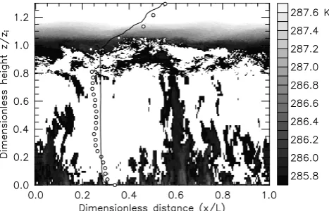
An overview of the boundary-layer structure is shown in Fig. 2, where contours of the e2 field in the range
285.7<e2<287.7 K are displayed in a (x,z) plane located
near an updraft at 15:00 EST. The mixed layer as well as the IL are strongly turbulent, implying that the thickness of the IL has a high variability. Fast-rising localized updrafts impact the IL (which leads to a folding of the interface) or erode the interface by a scouring mechanism. Similar down-ward plumes transport heat from the cooled sea surface to-ward the bottom of the oceanic mixed layer (D’Asaro et al., 2002). These entrainment events are localized and turbulent motions mix the entrained air downwards. The typical hori-zontal size of the convective cells atz/zi=0.25 is found to be
in the range 1500–2000 m, which is in good agreement with that found in previous studies (e.g. Schmidt and Schumann, 1989), and is in the order of the mixing depthzi.
To identify the instantaneous structure of these cells, we use theQ-criterion (Hunt et al., 1988). This criterion is de-rived from the second invariant of the fluctuating velocity gradient tensor∇
eu, denotedQ, which is expressed as Q=1
2 RgijgRij−SfijSfij
, (14)
Fig. 2. Visualization of the structure of the boundary layer using potential temperaturee2contours in a(x,z) plane located in the
vicinity of an updraft at 15:00 EST. The distances alongxandzare scaled by the domain lengthLand the mixed layer depthzi,
re-spectively. The grayscale color table indicatese2variations at the
interface (lower and higher2eappear white). The2eprofiles,
mea-sured during the Wangara experiment (◦) and computed from the LES results as a horizontally-averaged profile over the computa-tional domain (—), are also included for comparison.
wheregRij=(1/2) ∂juei−∂iuej
andSfijare the
antisymmet-ric and symmetantisymmet-ric parts of∇
eu, respectively. TheQ-criterion
may be regarded as the competition between the rotation rate
e
R2=
g
RijRgij and the strain rateSe2=SfijSfij. Thus, positive Qisosurfaces highlight areas where the rotation rate over-comes the strain rate, which are therefore eligible as vortex envelopes.
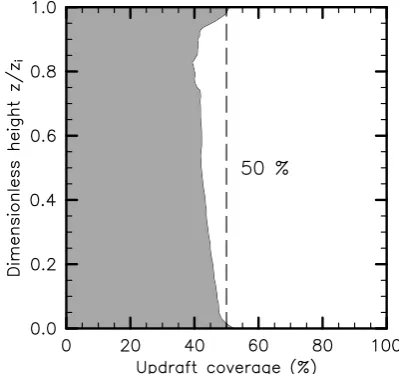
An isosurface ofQof positive value is displayed for an isolated convective cell pattern at 15:00 EST in Fig. 3a. The highlighted structures are traces of the fast rising updrafts, which are characterized by strong vorticity components. A horizontal cross-section of these updrafts is visible in Fig. 3b, where the vertical velocity scaled byw∗is plotted at the same time. It is then possible to discuss the degree of organiza-tion of the convective cells. They consist of well organized updrafts, which vanish and diffuse at the interface creating broad ring-shaped patterns. The air mass is gradually mixed downwards in the center of the pattern. Downdrafts are not organized compared to updrafts, and lead to downward mix-ing associated with small-scale turbulent structures. The fast rising updrafts occupy a smaller fraction (about 40%) of the CBL horizontal cross-sectional area than the slowly broader downdrafts (see Fig. 4), due to the vanishing of the verti-cal mass flux averaged over a horizontal surface. The val-ues of this fraction are consistent with observational data (Lenschow, 1998).
3.2 Mixed-layer statistics
The statistical properties of the mixed layer have been stud-ied in several papers (e.g. Moeng and Wyngaard, 1988;
Fig. 3. (a) Iso-surfaceQ=0.0015 s−2for an isolated convective cell at 15:00 EST. The displayed view encompasses a horizontal domain of about 1.5 km×1.5 km, the height ranging fromz=0 tozi. (b)
Contour plot of the dimensionless vertical velocity ew/w∗ at the
same time in the horizontal planez=zi/2. At the displayed time,
w∗=1.70 m s−1 andzi=1300 m. The contour lines correspond to e
w/w∗=±1,±2, ...Solid and dashed lines represent positive and negative contour values, respectively, with darkest zones being as-sociated with updrafts and lightest with downdrafts. The distances alongxandyare normalized by the domain lengthL. The structure visible in Fig. 3a has a horseshoe shape, which is clearly visible in Fig. 3b for approximately 0.2≤y≤0.6 and 0.2≤(−x/L+1)≤0.6.
Peltier et al., 1996; Kelly and Wyngaard, 2006), lead-ing to the conclusions that the kinetic energy density and temperature variance spectra obey Kolmogoroff and Corrsin-Oboukhov laws, respectively, the universal constants in these spectra being also recovered.
Our interest in this section is to show that the frequency spectrum for the horizontal velocity matches precisely the spatial one-dimensional longitudinal spectrum when a Tay-lor assumption, based upon transport of fluctuations by the convective cells, is made. The computation of the spatial and frequency spectra also provides the typical length and time scales, respectively, of the mixed layer.
Fig. 4. Relative spatial coverage of updrafts as a function ofz/zi,
as computed from the surface occupied by positive values of the vertical velocity.
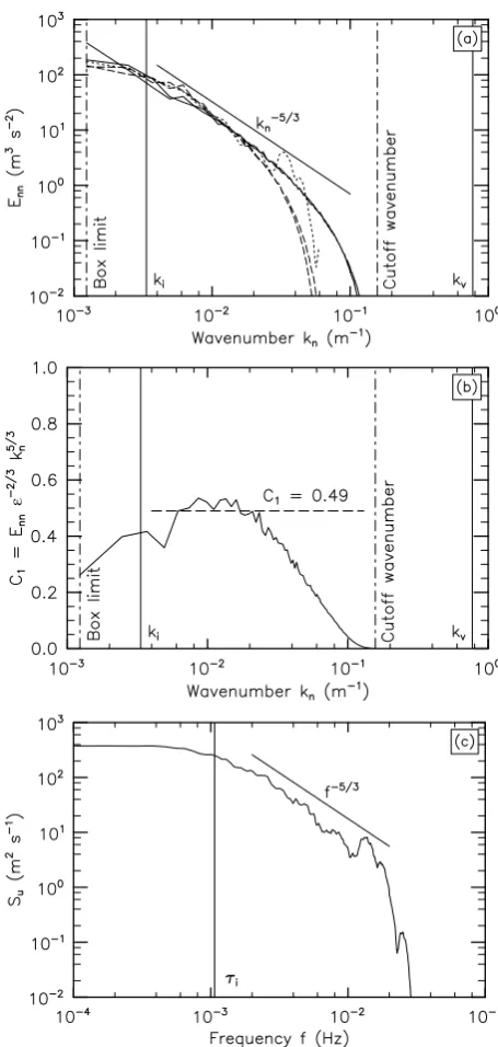
The one-dimensional longitudinal spectra of kinetic en-ergy density for eu and ev, denoted by Exx(kx,t ) and Eyy ky,t, respectively, are displayed in Fig. 5a. For
homo-geneous and isotropic turbulence, the spectra should behave as
Enn(kn,t )=C1ε2/3k −5/3
n , (15)
whereknis the wavenumber, the subscriptndenotingxory,
andC1=(18/55)CK≈0.49 forCK=1.5 (e.g. Champagne et al., 1977; Moeng and Wyngaard, 1988). The computed constantC1averaged for theeuandevcompensated spectra is
displayed versusknin Fig. 5b. The value ofC1thus obtained agrees well with the theoretical prediction of 0.49 for the smallest scales of the inertial range. We also note that these spectra are nearly the same, as expected from local isotropy. Two wavenumbers are indicated in Fig. 5a and b, denoted byki andkv. The former, ki, is the wavenumber at which
the two-dimensional spectra of u˜ andv˜ peak (not shown). Therefore`i=2π/ ki is the integral scale of turbulent
mo-tions. The latter,kv, is defined as 2π/`v, where`vis the
ef-fective dissipative scale, namely`v= νt3/
1/4
, withand νt being inferred from the SGS model. The computed
in-tegral scale`i is close to 1900 m, which corresponds to the
typical size of the convective cells. In the present LES, the dissipative scale`vis in the order of 5 m.
C. Chemel et al.: Estimating the diffusive heat flux across a stable interface forced by convective motions 193 power law, withf being the frequency of the motions, is
ex-pected in the inertial range for the velocity components. The frequency spectrum ofeu, denoted bySu(f ), computed from
12:00 EST to 15:00 EST atz=500 m in the center of the(x,y) plane, is displayed versusf in Fig. 5c. Af−5/3power law is obtained over almost a decade in the inertial range. Beyond f=0.03 s−1, turbulence is significantly damped by the SGS turbulent viscosity. This frequency corresponds to a charac-teristic time scale of 30 s, which is approximately the time for disturbances to travel across a grid element in the mesh.
The eddy-turnover time τi associated with the integral
scale`imay be estimated byτi=`i/eurms, whereeurmsis the
root-mean-square ofeu. This yields a time of 15 min, which is the typical time for air to circulate between the ground sur-face and the top of the mixed layer, namely roughlyzi/w∗,
as we checked it. The corresponding frequencyfi=2π/τi
is indicated in Fig. 5c.
Using the Taylor’s hypothesis, frequency spectra can be converted to one-dimensional wavenumber spectra by sub-stituting the frequency f for kx|eu|. The one-dimensional
wavenumber spectrum thus obtained is superimposed upon Enn in Fig. 5a. Both spectra remarkably coincide over the
inertial range. This demonstrates the reliability of the Tay-lor’s hypothesis within the mixed layer.
Thus, the turbulence within the mixed layer may be as-sumed to be locally homogeneous and isotropic over a broad range of scales in the inertial range. We checked that the IL is forced by the largest scales of the mixed layer by inves-tigating the vertical evolution of the two-dimensional heat flux spectrum, as done by Schmidt and Schumann (1989) from LES results and by Kaiser and Fedorovich (1998) from wind tunnel measurements. In agreement with these authors, we found that the heat flux spectrum becomes negative at the largest scales as the IL is approached from below (not shown). This implies that heat is transferred down from the IL and that the largest scales of the mixed layer are involved in this process.
4 Entrainment rate formulation
In this section, the focus is directed onto the IL where en-trainment events take place. As recalled in the introduction, the parameterization of the entrainment rate at the top of the CBL,we, involves the (unknown) heat fluxFi at the
inter-face and hence a closure for this flux. In this section, we show thatFi can be computed exactly from the method of
Winters et al. (1995). Then we introduce a turbulent ther-mal diffusivity fromFi, which we also compute by tracking
Lagrangian fluid particles within the interface. This analysis is finally applied to the “first-order” model discussed in the introduction.
We first compute the characteristics of the IL from our LES, which are needed in the analysis of entrainment.
Fig. 5. (a) One-dimensional longitudinal velocity spectraEii(ki)
ofeuandevcomputed for the 256
3resolution run (–) at 15:00 EST and averaged over the range 0.4<z/zi<0.6. The spectra computed
for a 1283resolution run (- - -) are superimposed for comparison. The dotted line (· · ·) represents the spectrum deduced from the fre-quency velocity spectrumSu(f )ofeu, displayed in plot (c) and
com-puted for the 2563resolution run, from 12:00 EST to 15:00 EST atz=500 m in the center of the(x,y)plane. (b) ConstantC1 in Eq. (15) computed for the 2563resolution run and averaged for the
euandevspectra as a function ofki.
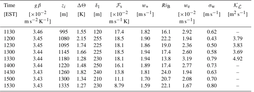
Table 1. Characteristics of the convective boundary layer for the 2563resolution run.
Time g β zi 12 δ1 Fs w∗ RiB we σw KL
[EST] [×10−2 [m] [K] [m] [×10−2 [m s−1] [×10−2 [m s−1] [m2s−1]
m s−2K−1] m s−1K] m s−1]
1130 3.46 995 1.55 120 17.4 1.82 16.1 2.92 0.62 –
1200 3.45 1080 2.15 255 18.5 1.90 22.2 1.94 0.43 3.79
1230 3.45 1095 1.74 225 18.1 1.86 19.0 2.36 0.50 3.83
1300 3.44 1145 1.66 225 18.5 1.94 17.4 2.60 0.58 3.69
1330 3.44 1180 1.28 230 18.1 1.94 13.8 3.19 0.79 4.92
1400 3.44 1220 1.48 250 16.1 1.89 17.4 2.77 0.73 –
1430 3.43 1260 1.82 240 13.8 1.81 24.0 1.94 0.63 –
1500 3.43 1300 1.34 210 11.1 1.70 20.7 2.08 0.70 –
1530 3.43 1335 1.27 230 8.79 1.59 22.1 1.67 0.80 –
4.1 Characteristics of the IL
Characteristics of the CBL are displayed in Table 1 for the 2563 resolution run, at successive times during the mixed layer growth. The mixing depth zi is defined as the level
where the heat flux is minimum as in the standard flux method (e.g. Fedorovich and Mironov, 1995; Sullivan et al., 1998). The values ofzi obtained in this way were compared
with those computed from the gradient method, described for instance by Sullivan et al. (1998), for whichzicorresponds to
the height above ground level where∂32eis maximum.
Rela-tive differences were found to be lower than 10%. The lower and upper limits of the IL were more difficult to determine. First, we have used computed values of the second deriva-tive∂322e. Indeed,∂32e2is expected to reach a maximum and
a minimum at the lower and upper limits of the IL, respec-tively. Since large∂32e2values often occur close to the ground
surface, it was computed fromzi upward and downward to
search the first minimum and maximum values, respectively. Nonetheless, this method was found to be not so accurate be-cause of non representative local extrema of∂32e2. Thus, the
thickness of the IL,δ1, was computed asz2−z1, wherez1 co-incides with the zero-crossing height of the heat flux profile andz2is the vertical position where the heat flux first goes to zero abovezi, as illustrated in Fig. 1a. Note that, consistent
with the convection tank measurements of Deardorff et al. (1980),δ1/zi is close to 0.2 for strong enough stratification
of the interface (see Table 1). The potential temperature jump 12was calculated ase2(z2)−e2(z1). The entrainment ve-locity was computed from the time derivative ofzi using a
centered difference scheme.
4.2 Computing the diffusive heat flux at the interface
Mixing results from a diffusive heat flux. Indeed, a purely advective heat flux displaces thee2 surfaces without
mod-ifying their value. The diffusive heat flux occurs across,
and normal to, the constante2surfaces (since there cannot be
any diffusive flux along those surfaces).
One way to compute the diffusive heat flux is to average the actual advective heat flux in space or time. The idea in doing so is that the oscillations due to reversible (wave) mo-tions are filtered out by the averaging process and the residual non zero value gives the diffusive flux. However this method is not very precise because the residual value is usually very small relative to the maximum advective flux. An alternative method to access directly this residual diffusive contribution is provided by Winters et al. (1995). The principle of this method is to compute the hydrostatic equilibrium tempera-ture profile associated with the minimum potential energy of the fluid at a given time. Conceptually this equilibrium state is reached by moving adiabatically and instantaneously the fluid particles towards their hydrostatic equilibrium position. Let2es(z,t ) be the temperature profile of this virtual equi-librium state, which is stable by construction. e2s evolves in time because of diffusive processes only and satisfies an equation of the form:∂t2es= −∂3ϕd. The fluxϕdis respon-sible for the temporal variation ine2sand is therefore the dif-fusive heat flux responsible for mixing. Hence, in the present context of interfacial mixing by convective motions,
ϕd=F, for z1< z < z2. (16)
In practice, the stable temperature profilee2s(z,t )at a given time is computed by a simple adiabatic sorting of the tem-perature field at that time. More precisely the2es profile is retrieved from each instantaneous e2field as follows. Let
us consider a volumeV, fixed with time, extending on both sides of the interface, from a level above the ground surface (atz/zi=0.5) up to a level far above the upper boundary
of the IL (atz/zi=1.5). The instantaneous2eprofiles are
C. Chemel et al.: Estimating the diffusive heat flux across a stable interface forced by convective motions 195 being the coldest2. Then, the change in time of the
result-ing sorted profile gives access to the diffusive heat flux. As shown by Winters et al. (1995),ϕdhas the following theoret-ical expression
ϕd(z,t )= − hκt
∇e2
2 iI ∂32es
, (17)
wherehiI denotes an average along ae2-surface andκt is
the SGS turbulent diffusivity. Note thatϕdis negative as ex-pected. If pure laminar diffusion occurs, Eq. (17) reduces to the standard flux-gradient relationϕd,lam= −κ ∂3e2s, where κ is the molecular diffusivity. Equation (17) therefore pro-vides an expression to compute the turbulent diffusive flux ϕdat any time.
To examine whether the horizontally averaged heat flux of the resolved scalesFe=we02e0is a good approximation of the
diffusive heat flux, we compare its value with that given by Eq. (17). For consistency with the definition of the interfacial heat flux, we should compareFeandϕdat the altitudes where they each reach a minimum value, namely atz=zi∗, say, for ϕdand atz=zi forFe. IfFeis a good approximation forϕd, these minimum values as well asz∗i andzi should be very
close.
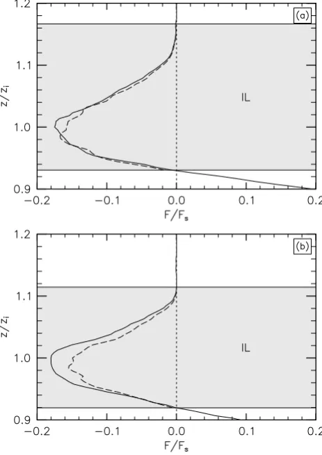
The vertical profiles ofFeandϕdare compared in Fig. 6 at 12:00 EST and 13:30 EST. The fluxϕdis negative, by def-inition, and is slightly smaller thanFe: the minimum value
of ϕd is 5% smaller than that of Feat 12:00 EST and 16%
smaller at 13:30 EST. The altitude z∗i whereϕd reaches its absolute minimum is 20 m lower thanzi, the relative
differ-ence in altitude being less than 2%. This shows thatwe02e0(zi)
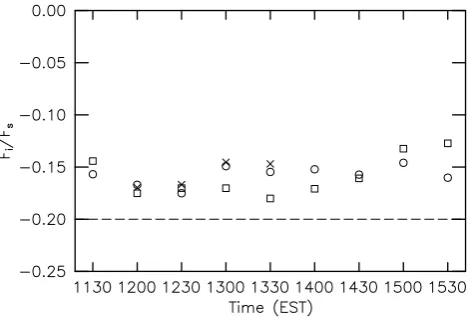
is a very good approximation for the diffusive heat flux at the interface. In the following we takeϕd z∗i as the reference
value for this flux. In other words, we defineFi byϕd z∗i
. We now compare the values ofwe02e0(zi)andϕd z∗iscaled by the surface heat flux for the times displayed in Table 1 (see Fig. 7). The constant value –0.2 is also indicated since a commonly used closure forFi is that it is proportional to Fs with an empirical –0.2 coefficient. (The heat flux based upon the Lagrangian turbulent diffusivity, discussed in the next section, is also displayed in Fig. 7.) Figure 7 shows that the good agreement found between the two fluxes in Fig. 6 holds at all times, regardless of the value of the Richard-son number, the relative difference ranging between 3% and 2Incompressibility is assumed in the sorting method and we checked that this assumption is verified here. Indeed, the vertical displacements of fluid particles in the sorting process are at most equal to the thickness of the interfacial layer, that is 250 m or so. Since the sorting process is adiabatic, the change in the volumeV of the fluid particles before (state 1) and after (state 2) sorting can be estimated by writing thatp1.V1γ=p2.V2γ, whereγ=1.4 is the heat capacity ratio. If one assumes that the pressure is dominated by its hydrostatic component, one finds that the change in volume of the fluid particles during the sorting process is at most 3%.
Fig. 6. Vertical profile of the heat fluxeswe0f20(–) andϕd( - - - )
scaled by the surface heat fluxFsat 12:00 EST (a) and at 13:30 EST (b), as a function of the vertical coordinatezscaled byzi. The filled
area represents the interfacial layer (IL).
20%. Note thatϕd zi∗/Fsvaries by at most 9% during the 4 h of simulation reported here whilewe02e0(zi)/Fs changes twice more. Hence, not surprisingly, the diffusive heat flux is much less sensitive to large scale fluctuations than the ad-vective heat flux. Figure 7 also shows that the simple closure
Fs= −0.2Fs is an acceptable lower bound of the diffusive heat flux at the IL during this period of time.
4.3 Estimate of mixing from the turbulent diffusivity
4.3.1 Computation of the turbulent diffusivity fromϕd
A turbulent diffusivityKϕ can be inferred from the turbulent
diffusive heat fluxϕd, namely
ϕd(z,t )= −Kϕ∂3f2s. (18)
Note that, using Eq. (17) forϕd, Kϕ can also be expressed
directly in terms of the temperature field. If the scale of the vertical gradient of2fs is much larger than the turbulent overturning scale, relation (18) is linear i.e.Kϕ is (nearly)
Fig. 7. The turbulent diffusive heat flux at the interfaceFi (scaled
byFs) computed by different methods, for the times indicated in Table 1: byϕd(z∗i)(◦); bywe0f20(zi)(); by Eq. (18) atz=z∗
i,
us-ing the turbulent diffusivityKLaveraged over the interfacial layer (×); by−0.2Fs(dashed line).
uniform inz(e.g. Gregg, 1987). Under this condition, the turbulence may be assumed locally homogeneous.
The turbulent overturning scale within the IL is usually quantified by the buoyancy length scale`b, defined by the ratio of the rms fluctuating vertical velocityσwand the buoy-ancy frequency (e.g. Hopfinger, 1987). `bis the largest ver-tical distance a fluid particle can move in a stably-stratified fluid against the potential temperature gradient. We com-puted`bfor the times indicated in Table 1, using the rms ver-tical velocity with the mean referring to an average over the IL (see Table 1) and using the buoyancy frequency defined asNB=(g β 12/δ1)1/2. We found that`bvaries between 25 and 58 m, with a mean value of 41 m. This is consistent with the analysis of the IL dynamics by Otte and Wyngaard (2001), which yields`b≈20 m for conditions close to our LES (see their cases 19 to 22, in which12is twice stronger than in the present case, all parameters being otherwise com-parable). The values of`bthat we found have to be compared with the length scale associated with the mean vertical gradi-ent ofe2, which isδ1. Sinceδ1≈225 m in our LES (see Ta-ble 1), local homogeneity may be assumed.
We computed Kϕ from our LES during the regime of
equilibrium entrainment, which lasts from 12:00 EST to 13:30 EST as the ground surface heat flux is nearly constant during this period (see the values ofFs in Table 1). Dur-ing this period, the values ofKϕ obtained from Eq. (18) (and
averaged over the IL) are between 3.52 and 4.17 m2s−1 de-pending upon time, and average 3.8 m2s−1. In terms of SGS turbulent diffusivity κt, we found that Kϕ is in the range
10–25κt, implying that the IL is turbulent.
4.3.2 Computation of the turbulent diffusivity from the dispersion of particles
An alternative method, based upon the dispersion of fluid particles within the IL, can be used to retrieve the turbulent diffusivity. This diffusivity will be denotedKLhereafter to make it distinct from that computed fromϕd(though we ex-pectKL'Kϕ). By “fluid particles”, as usual, we mean non
buoyant particles, which are advected by the velocity field (see Eq. 9).
Let(δz)ms(t )be the mean square vertical displacement of fluid particles at timetfor a given release of a particle cloud. (δz)ms(t )is defined by
(δz)ms(t )= 1/Np
Np
X
n=1
[zn(t )−zG(t )]2, (19)
whereNp is the number of particles of the release,zn(t )is
the vertical position of the particlenandzG(t )the vertical position of the center of gravity of the particle cloud at time t. If the turbulence is locally homogeneous and stationary, and fort≥2TL, withTLbeing the Lagrangian time scale of the turbulence,KL can be inferred from the growth rate of (δz)ms(see Taylor, 1921; Hunt, 1985, for a review), namely
dt(δz)ms=2KL. (20)
Since the IL is continuously forced by the quasi-stationary convective cells, the turbulence within this layer may be as-sumed stationary. In this case, the Lagrangian time scale
TL is in the same order of magnitude as the Eulerian time scaleTE(e.g. Hanna, 1981; Yeung, 2002; Dosio et al., 2005). This result is valid also in the presence of a stable stratifica-tion (Hunt, 1985). Let us assume thatTE=2π/NB. Hence,
TE≈40 s implying that 2TLis in the order of 1 min.
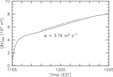
Particles were released forz−zi=±100 m, that is, within
the bulk of the IL. Note that some of the particles were released below and above the IL since its thickness varies over a wide range within the computational domain. The re-leases were made at 4 equally-spaced times from 11:55 EST to 13:25 EST over 10-min periods and resulted in a total of 57 500 particles per release. As an example, the time evolu-tion of(δz)msfor the release carried out around 12:00 EST is displayed in Fig. 8. A quasi-linear growth occurs after about 1 min, whose growth rate is 2KLaccording to Eq. (20). Val-ues forKLbetween 3.24 and 3.83 m2s−1were obtained de-pending upon the time of the release and average 3.6 m2s−1. This range of values forKLis in very good agreement with that computed for Kϕ from the diffusive heat flux, the
rel-ative differences being lower than 10% on average. This is attested in Fig. 7 where−KL∂3f2sscaled byFsis displayed at altitudez∗i for the times reported in Table 1: the relative difference withϕd z∗i
is at most 5%.
C. Chemel et al.: Estimating the diffusive heat flux across a stable interface forced by convective motions 197
Fig. 8. Time evolution of(δz)ms(t )and resulting turbulent diffu-sivityKLat 12:00 EST. The dashed line corresponds to the least-square curve fit of(δz)ms(t ), which is used to estimateKL.
SGS turbulence is likely to contribute to dispersion within the IL where small-scale turbulence dominates and TL is rather small. Thus, we conducted a simulation with a single release at 11:55 EST and switched off the SGS contribution in the Lagrangian stochastic model. In this case,(δz)mswas found to increase less rapidly during 1−2TL but reached a quasi-linear regime with the same slope (not shown), giving the same value ofKL. Therefore the SGS contribution ap-pears to play a negligible role in dispersing the particles. This result is consistent with the findings of Gopalakrishnan and Avissar (2000), and Cai et al. (2006) for a passive tracer.
4.4 Application to the “first-order” model
4.4.1 Evaluation of the “first-order” model
Within the framework of the “first-order” jump model pro-posed by Betts (1974), the entrainment heat flux at the inter-faceFi is related to the entrainment rate by
−Fi=we12−δi∂t2∗, (21)
whereδi=z2−zi and2∗=2(ze i)+e2(zi+δ)/2. In the
limit of infinitely small thickness of the IL, i.e. δi→0,
Eq. (21) reduces to the “zero-order” approximation for the interfacial heat flux derived by Lilly (1968), namely−Fi= we12.
Our purpose in this subsection is to evaluate the first-order model forweby comparing the LES computation ofwefrom its definition (namely dtzi) with its prediction by Eq. (21)
using Fi =ϕd z∗i. In order to compare also with the
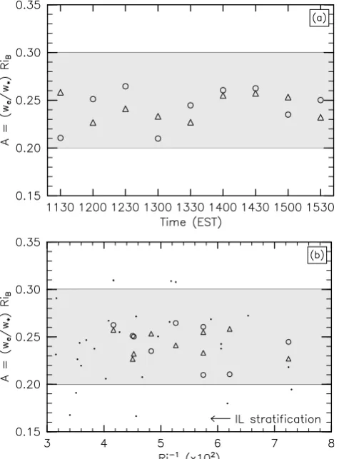
ex-perimental data of Deardorff et al. (1980) we rather consider the parameterA=(we/w∗)RiBinstead ofwe. This param-eter is plotted in Fig. 9 versus time (see Fig. 9a) and versus RiB−1 (see Fig. 9b) for the times reported in Table 1. The
convection tank measurements of Deardorff et al. (1980) are included in Fig. 9b. The two quantitiesw∗andRiBare com-puted from the LES.
A very good agreement is obtained between the LES val-ues ofweand its prediction by the first-order model, the rel-ative difference forAranging between 2% and 18% with a mean value of 8%. (The relative difference forAwith−Fi
computed aswe02e0(zi)averages 11%.) The parameterAis
in the range 0.21–0.26 and averages 0.24, which is in good agreement with values reported in previous studies. This also shows that the standard parameterizationwe/w∗=0.2RiB−1 for the entrainment rate is consistent with the present anal-ysis of mixing. The coefficientAwas shown to be equal to the efficiency of the mixing process by Chemel and Staquet (2007).
As pointed out by Fedorovich et al. (2004), the computa-tion of the different terms in a given model should be con-sistent with the model order. The “first-order” model re-lies upon the finite thickness of the IL. ReplacingFi byϕd, whose computation involves the depth of the CBL through the sorting process, may not fulfill this consistency condition. However, the temperature profile being (quasi-) uniform in the mixed layer and stable above the IL, this sorting process involves actually only the thickness of the mixed layer (see Fig. 6). Hence, estimatingFi byϕd z∗iin Eq. (21) is con-sistent with a “first-order” model.
4.4.2 Expression of the “first-order” model in terms of the turbulent diffusivity
WithFi=ϕd z∗i, Eq. (18) becomes
Fi= −Kϕ∂3f2s zi∗
. (22)
Approximating∂32fs z∗iby12/δ1, the “first-order” model (21) becomes
we=K/δ1+δi∂t2∗/12, (23)
where K=Kϕ or KL. The approximation ∂32fs z∗i
' 12/δ1 should be discussed. The relative differences be-tween∂32es z∗iand∂32(ze i)were found to be less that 5%
in our simulation. The relative differences between∂3e2(zi)
and 12/δ1 range from 6% to 27% while those between ∂32(ze i)and 12/δi range from 14% to more than 100%.
Hence,12/δ1is a better approximation of∂32(ze i)than is 12/δi.
It is worth noting that by introducingδ1in Eq. (23), we extend the “first-order” model beyond that proposed by Betts (1974). Equation (23) is actually a mixture between what Sun and Wang (2008) have called the models “FOM1” and “FOM2”, which differ only in the definition of the IL thick-ness (equal toδiand toδ1, respectively). With this expression forweandK=KL, the parameterA=(we/w∗)RiBis plot-ted in Fig. 10 versusRiB−1. These values are compared with those obtained when we is computed from the LES by its
Fig. 9. (a) Dimensionless parameterA=(we/w∗)RiBfor the dif-ferent times displayed in Table 1, withwecomputed by two meth-ods: from the LES (using its definitiondtzi) (4); from the
first-order model withFi=ϕd z∗i (◦). (b) same as (a) except that (we/w∗) RiBis now plotted as a function ofRiB−1. Convection tank measurements of Deardorff et al. (1980) are included for com-parison (·). The filled area representsAin the range 0.2–0.3.
definition (we=dtzi). A very good agreement is found, the
relative difference being lower than 10% on average. Also plotted in Fig. 10 are the results from a simple expression for we, namely
we=KL/δ1. (24)
It is well-known (Sullivan et al., 1998) that the term δi∂t2∗/12in the “first-order” model is not negligible
com-pared to−Fi/12in the range ofRiBvalues considered in our LES, its contribution here being up to 40% for the lowest RiBvalues. However, Fig. 10 shows that, when the stratifica-tion is strong enough (RiBapproximately larger than 15 ac-cording to our data), the simple expression (24) accounts for the actual value of the entrainment rate to better than 25%.
Fig. 10. Dimensionless parameterA=(we/w∗)RiBfor the differ-ent times displayed in Table 1 as a function ofRiB−1. weis com-puted by three methods: from the LES (using its definitiondtzi)
(4); from Eq. (23), withK=KLaveraged over the interfacial layer (×); by the simple model (24) (). Convection tank measurements of Deardorff et al. (1980) are included for comparison (·). The filled area representsAin the range 0.2–0.3.
5 Concluding remarks
In the present paper, the entrainment at the top of the convectively-driven boundary layer is reexamined using data from a high-resolution LES initialized by a commonly used sounding of Day 33 of the Wangara experiment and the anal-ysis of mixing proposed by Winters et al. (1995). Note than an analysis along the same lines was conducted by D’Asaro et al. (2002) for the oceanic convective mixed layer.
The mixed layer turbulence which forces the IL is first analysed in the present case of a “realistic” initialization. We found that the turbulence follows precisely the Kolmogorov spectral law for the velocity field over almost a decade in the inertial range. The multiplicative constant in this law is found to be in good agreement with previous measurements in the atmosphere. The Kolmogorov spectral law also holds for the frequency spectrum, when the Taylor’s frozen turbulence hy-pothesis is used. To our knowledge, this is the first time that this hypothesis is verified properly in the context of the at-mospheric boundary layer. Hence, the turbulence within the mixed layer may be assumed to be locally homogeneous and isotropic over a broad range of scales in the inertial range.
This turbulence forces and mixes the IL at the top of the convective layer. The parameterization of the heat flux at the IL, which is responsible for mixing, and of the resulting en-trainment rate has been the subject of intensive research since Lilly (1968). We showed that the heat flux at the IL can be computed exactly from the analysis of Winters et al. (1995). The exact expression of this flux is denotedϕd. We defined the heat flux at the interface, usually referred to asFi, by the
C. Chemel et al.: Estimating the diffusive heat flux across a stable interface forced by convective motions 199 in the atmospheric context) and we denotedz∗i the altitude
at which this minimum value is reached. This allowed us to show that the standard closure forFi, namely the minimum
value of the horizontally averaged advective heat flux, agrees well withϕd z∗i, to about 10%.
The exact computation ofFialong with a properly defined
temperature profile within the interface (namely through a “sorting” process, following Winters et al., 1995) naturally yields a turbulent thermal diffusivity. The values of this tur-bulent diffusivity were recovered from the dispersion of fluid particles within the IL, which were tracked by a Lagrangian stochastic model coupled with the LES. The values thus de-rived agree indeed to better than 10% on average with those computed fromϕd(whether SGS turbulence is included or not in the Lagrangian stochastic model).
These different estimates for the interfacial heat fluxFi
were next applied to the parameterization of the entrainment ratewewithin the framework of the “first-order” model. This model basically relies on the thickness of the IL (as opposed to the “zero-order” model, where this thickness is infinitely small) and provides an expression forweinvolving bothFi
and the thickness of the IL. We examined different predic-tions forwe from this model, depending upon the estimate forFi, which we compared with the LES value ofwe. Over-all, whetherFiis computed from its exact expressionϕd z∗i
, from its approximation using the horizontally-averaged ad-vective heat flux or when the Lagrangian turbulent diffusiv-ity is introduced, the prediction ofwe by the “first-order” model agrees to about 10% with that computed from the LES using its definition (the best agreement being found for
Fi=ϕd z∗i).
A simple expression was also proposed for the entrainment rate, for whichweis equal to the Lagrangian turbulent dif-fusivity divided by the IL thickness. We showed that the values thus obtained differ from the LES values by 25% for strong enough stratification only (this relative difference be-ing larger otherwise). However, for this expression to be of any use, one needs to access both the IL thickness and the turbulent diffusivity. Remote sensing techniques can provide values of the IL thickness (e.g. Steyn et al., 1999; Cohn and Angevine, 2000). Measurement of the turbulent diffusivity is likely to be more difficult but, as discussed by Winters and D’Asaro (1996), its values can still be retrieved from finescale-resolving vertical temperature profiles.
Acknowledgements. All the major computations were performed thanks to the “Institut du D´eveloppement et des Ressources en Informatique Scientifique” (IDRIS), and the “Centre Informatique National de l’Enseignement Sup´erieur” (CINES) computing re-sources. We wish to thank I. Vinkovic, C. Aguirre, and S. Simo¨ens for providing us with a part of the Lagrangian stochastic model.
Edited by: V. Shrira
Reviewed by: two anonymous referees
References
Betts, A. K.: Reply to comment on the paper “Non-precipitating cumulus convection and its parameterization”, Q. J. Roy. Me-teor. Soc., 100, 469–471, 1974.
Bretherton, C. S., MacVean, M. K., Bechtold, P., Chlond, A., Cot-ton, W. R., Cuxart, J., Cuijpers, H., Khairoutdinov, M., Koso-vic, B., Lewellen, D., Moeng, C.-H., Siebesma, P., Stevens, B., Stevens, D. E., Sykes, I., and Wyant, M. C.: An inter-comparison of radiatively driven entrainment and turbulence in a smoke cloud, as simulated by different numerical models, Q. J. Roy. Meteor. Soc., 125, 391–423, 1999.
Cai, X., Zhang, R., and Li, Y.: A large-eddy simulation and La-grangian stochastic study of heavy particle dispersion in the con-vective boundary layer, Bound.-Lay. Meteorol., 120, 413–435, 2006.
Cai, X.-M. and Luhar, A. K.: Fumigation of pollutants in and above the entrainment zone into a growing convective boundary layer: a large-eddy simulation, Atmos. Environ., 36, 2997–3008, 2002. Champagne, F. H., Friehe, C. A., LaRue, J. C., and Wyngaard, J. C.: Flux measurements, flux estimation techniques, and fine-scale turbulence measurements in the unstable surface layer over land, J. Atmos. Sci., 34, 515–530, 1977.
Chemel, C. and Staquet, C.: A formulation of convective entrain-ment in terms of mixing efficiency, J. Fluid Mech., 580, 169–178, 2007.
Clarke, R. H., Dyer, A. J., Brook, R. R., Reid, D. G., and Troup, A. J.: The Wangara experiment: Boundary layer data, Tech. Paper 19, CSIRO Atmospheric Research, Aspendale, Australia, 362 pp., 1971.
Cohn, S. A. and Angevine, W. M.: Boundary layer height and en-trainment zone thickness measured by lidars and wind-profiling radars, J. Appl. Meteorol., 39, 1233–1247, 2000.
D’Asaro, E. A., Winters, K. B., and Lien, R.-C.: Lagrangian analy-sis of a convective mixed layer, J. Geophys. Res., 107(C5), 3040, doi:10.1029/2000JC000247, 2002.
Deardorff, J. W.: Stratocumulus-capped mixed layers derived from a three-dimensional model, Bound.-Lay. Meteorol., 18, 495–527, 1980.
Deardorff, J. W., Willis, G. E., and Stockton, B. H.: Laboratory studies of the entrainment zone of a convectively mixed layer, J. Fluid Mech., 100, 41–64, 1980.
Dosio, A., Vil´a-Guerau de Arellano, J., Holtslag, A. A. M., and Builtjes, P. J. H.: Relating Eulerian and Lagrangian statistics for the turbulent dispersion in the atmospheric convective boundary layer, J. Atmos. Sci., 62, 1175–1191, 2005.
Fedorovich, E., Conzemius, R., and Mironov, D.: Convective entrainment into a shear-free, linearly stratified atmosphere: bulk models reevaluated through large eddy simulations, J. At-mos. Sci., 61, 281–295, 2004.
Fedorovich, E. E. and Mironov, D. V.: A model for a shear-free convective boundary layer with parameterized capping inversion structure, J. Atmos. Sci., 52, 83–95, 1995.
Fernando, H. J. S.: Turbulent mixing in stratified fluids, Annu. Rev. Fluid Mech., 23, 455–493, 1991.
Gopalakrishnan, S. G. and Avissar, R.: An LES study of the im-pacts of land surface heterogeneity on dispersion in the convec-tive boundary layer, J. Atmos. Sci., 57, 352–371, 2000. Gregg, M. C.: Diapycnal mixing in the thermocline: a review,
J. Geophys. Res., 92(C5), 5249–5286, 1987.
Hanna, S. R.: Lagrangian and Eulerian time-scale relations in the daytime boundary layer, J. Appl. Meteorol., 20, 242–249, 1981. Hannoun, I. A. and List, E. J.: Turbulent mixing at a shear-free
density interface, J. Fluid Mech., 189, 211–234, 1988.
Hong, S.-Y., Noh, Y., and Dudhia, J.: A new vertical diffusion package with an explicit treatment of entrainment processes, Mon. Weather Rev., 134, 2318–2341, 2006.
Hopfinger, E. J.: Turbulence in stratified fluids: a review, J. Geo-phys. Res., 92(C5), 5287–5303, 1987.
Hunt, J. C. R.: Diffusion in the stably stratified atmospheric bound-ary layer, J. Clim. Appl. Meteorol., 24, 1187–1195, 1985. Hunt, J. C. R., Wray, A. A., and Moin, P.: Eddies, stream and
con-vergence zones in turbulent flows, Report CTR-S88, Center For Turbulence Research, Stanford, CA, USA, 193–208, 1988. Kaiser, R. and Fedorovich, E.: Turbulence spectra and
dissipa-tion rates in a wind tunnel model of the atmospheric convective boundary layer, J. Atmos. Sci., 55, 580–594, 1998.
Kelly, M. and Wyngaard, J. C.: Two-dimensional spectra in the at-mospheric boundary layer, J. Atmos. Sci., 63, 3066–3070, 2006. Lamb, R. G.: A numerical simulation of dispersion from an ele-vated point source in the convective planetary boundary layer, Atmos. Environ., 12, 1297–1304, 1978.
Lenschow, D. H.: Observations of clear and cloud-capped convec-tive boundary layers, and techniques for probing them, in: Buoy-ant Convection in Geophysical Flows, edited by: Plate, E. J., Fedorovich, E., Viegas, D. X., and Wyngaard, J. C., Kluwer Academic Publishers, Dordrecht, The Netherlands, NATO ASI Series C: Mathematical and Physical Sciences, 513, 185–206, 1998.
Lesieur, M. and M´etais, O.: New trends in large-eddy simulations of turbulence, Annu. Rev. Fluid Mech., 28, 45–82, 1996. Lewellen, D. C. and Lewellen, W. S.: Large-eddy boundary layer
entrainment, J. Atmos. Sci., 55, 2645–2665, 1998.
Lilly, D. K.: Models of cloud-topped mixed layers under a strong inversion, Q. J. Roy. Meteor. Soc., 94, 292–309, 1968.
Linden, P. F.: The deepening of a mixed layer in a stratified fluid, J. Fluid Mech., 71, 385–405, 1975.
Manins, P. C. and Turner, J. S.: The relation between the flux ratio and energy ratio in convectively mixed layers, Q. J. Roy. Me-teor. Soc., 104, 39–44, 1978.
Matthews, P. C. and Cox, S. M.: Pattern formation with a conserva-tion law, Nonlinearity, 13, 1293–1320, 2000.
Moeng, C.-H. and Wyngaard, J. C.: Spectral analysis of large-eddy simulations of the convective boundary layer, J. Atmos. Sci., 45, 3573–3587, 1988.
Noilhan, J. and Planton, S.: A simple parametrization of land sur-face processes for meteorological models, Mon. Weather Rev., 117, 536–549, 1989.
Otte, M. J. and Wyngaard, J. C.: Stably stratified interfacial-layer turbulence from large-eddy simulation, J. Atmos. Sci., 58, 3424– 3442, 2001.
Peltier, L. J., Wyngaard, J. C., Khanna, S., and Brasseur, J. G.: Spectra in the unstable surface layer, J. Atmos. Sci., 53, 49–61, 1996.
Pleim, J. E. and Xiu, A.: Development and testing of a surface flux and planetary boundary layer model for application in mesoscale models, J. Appl. Meteorol., 34, 16–32, 1995.
Schmidt, H. and Schumann, U.: Coherent structure of the con-vective boundary layer derived from large-eddy simulations, J. Fluid Mech., 200, 511–562, 1989.
Sorbjan, Z.: Effects caused by varying the strength of the capping inversion based on a large eddy simulation model of the shear-free convective boundary layer, J. Atmos. Sci., 53, 2015–2024, 1996.
Stevens, B. and Lenschow, D. H.: Observations, experiments, and large eddy simulation, B. Am. Meteorol. Soc., 82, 283–294, 2001.
Steyn, D. G., Baldi, M., and Hoff, R. M.: The detection of mixed layer depth and entrainment zone thickness from lidar backscat-ter profiles, J. Atmos. Ocean. Tech., 16, 953–959, 1999. Sullivan, P. P., Moeng, C.-H., Stevens, B., Lenschow, D. H., and
Mayor, S. D.: Structure of the entrainment zone capping the con-vective atmospheric boundary layer, J. Atmos. Sci., 55, 3042– 3064, 1998.
Sun, J. and Wang, Y.: Effect of the entrainment flux ratio on the relationship between entrainment rate and convective Richardson number, Bound.-Lay. Meteorol., 126, 237–247, 2008.
Taylor, G. I.: Diffusion by continuous movements, Proc. Lon-don Math. Soc., 20, 196–212, 1921.
Taylor, G. I.: The spectrum of turbulence, P. Roy. Soc. Lond. A Mat., 164, 476–490, 1938.
Thomson, D. J.: Criteria for the selection of stochastic models of particle trajectories in turbulent flows, J. Fluid Mech., 180, 529– 556, 1987.
Vinkovic, I., Aguirre, C., and Simo¨ens, S.: Large-eddy simulation and Lagrangian stochastic modeling of passive scalar dispersion in a turbulent boundary layer, J. Turbul., 7, No. 30, 2006. Weil, J. C., Sullivan, P. P., and Moeng, C.-H.: The use of
large-eddy simulations in Lagrangian particle dispersion models, J. At-mos. Sci., 61, 2877–2887, 2004.
Winters, K. B. and D’Asaro, E. A.: Diascalar flux and the rate of fluid mixing, J. Fluid Mech., 317, 179–193, 1996.
Winters, K. B., Lombard, P. N., Riley, J. J., and D’Asaro, E. A.: Available potential energy and mixing in density-stratified fluids, J. Fluid Mech., 317, 115–128, 1995.
Xue, M., Droegemeier, K. K., and Wong, V.: The Advanced Regional Prediction System (ARPS) – A multi-scale non hy-drostatic atmospheric simulation and prediction model. Part I: Model dynamics and verification, Meteorol. Atmos. Phys., 75, 161–193, 2000.
Xue, M., Droegemeier, K. K., Wong, V., Shapiro, A., Brewster, K., Carr, F., Weber, D., Liu, Y., and Wang, D.: The Advanced Regional Prediction System (ARPS) – A multi-scale non hydro-static atmospheric simulation and prediction tool. Part II: Model physics and applications, Meteorol. Atmos. Phys., 76, 143–165, 2001.