www.clim-past.net/11/115/2015/ doi:10.5194/cp-11-115-2015
© Author(s) 2015. CC Attribution 3.0 License.
Simulating ice core
10
Be on the glacial–interglacial timescale
C. Elsässer1, D. Wagenbach1,†, I. Levin1, A. Stanzick1, M. Christl2, A. Wallner3, S. Kipfstuhl4, I. K. Seierstad5,
H. Wershofen6, and J. Dibb7
1Institut für Umweltphysik, University of Heidelberg, Im Neuenheimer Feld 229, 69120 Heidelberg, Germany 2Laboratory for Ion Beam Physics, ETH Zurich, 8093 Zurich, Switzerland
3Vienna Environmental Research Accelerator, University of Vienna, 1090 Vienna, Austria 4Alfred Wegener Institute for Polar and Marine Research, 27570 Bremerhaven, Germany 5Centre for Ice and Climate, University of Copenhagen, 2100-Copenhagen, Denmark 6Physikalisch-Technische Bundesanstalt, 38116 Braunschweig, Germany
7Institute for the Study of Earth, Oceans, and Space, University of New Hampshire, Durham, NH 03824, USA †deceased, 4 December 2014
Correspondence to: C. Elsässer ([email protected])
Received: 29 January 2014 – Published in Clim. Past Discuss.: 26 February 2014
Revised: 25 November 2014 – Accepted: 7 December 2014 – Published: 3 February 2015
Abstract. 10Be ice core measurements are an important
tool for paleoclimate research, e.g., allowing for the recon-struction of past solar activity or changes in the geomag-netic dipole field. However, especially on multi-millennial timescales, the share of production and climate-induced variations of respective 10Be ice core records is still up for debate. Here we present the first quantitative clima-tological model of the 10Be ice concentration up to the glacial–interglacial timescale. The model approach is com-posed of (i) a coarse resolution global atmospheric transport model and (ii) a local 10Be air–firn transfer model. Exten-sive global-scale observational data of short-lived radionu-clides as well as new polar 10Be snow-pit measurements are used for model calibration and validation. Being specif-ically configured for 10Be in polar ice, this tool thus al-lows for a straightforward investigation of production- and non-production-related modulation of this nuclide. We find that the polar10Be ice concentration does not immediately record the globally mixed cosmogenic production signal. Us-ing geomagnetic modulation and revised Greenland snow accumulation rate changes as model input, we simulate the observed Greenland Summit (GRIP and GISP2) 10Be ice core records over the last 75 kyr (on the GICC05modelext timescale). We show that our basic model is capable of re-producing the largest portion of the observed10Be changes. However, model–measurement differences exhibit multi-millennial trends (differences up to 87 % in case of
nor-malized to the Holocene records) which call for closer in-vestigation. Focusing on the (12–37) b2k (before the year AD 2000) period, mean model–measurement differences of 30 % cannot be attributed to production changes. However, unconsidered climate-induced changes could likely explain the model–measurement mismatch. In fact, the10Be ice con-centration is very sensitive to snow accumulation changes. Here the reconstructed Greenland Summit (GRIP) snow ac-cumulation rate record would require revision of+28 % to solely account for the (12–37) b2k model–measurement dif-ferences.
1 Introduction
the related solar and geomagnetic activity (Beer et al., 1988; Raisbeck et al., 1990; Bard et al., 1997; Muscheler et al., 2005; Vonmoos et al., 2006; Muscheler et al., 2007; Stein-hilber et al., 2012). However, due to aerosol-related transport and deposition processes of10Be, respective ice core records also hold information on past climate variability making this cosmogenic radionuclide also a valuable tool for estimating past snow accumulation rate changes (Mazaud et al., 1994; Steig, 1996; Wagner et al., 2001b). The question of whether to use10Be ice concentration records as proxy for production or climate variability depends on the timescale under inves-tigation as well as on the local climate conditions of the con-cerned drilling site. In either case, the detailed understanding of production- and non-production-related influences on the polar10Be ice concentration is an important requirement for the interpretation of the10Be ice core records.
In recent years, several studies improved the knowledge on processes which influence atmospheric10Be in polar regions. Atmospheric production rates have been calculated within elaborative Monte Carlo simulations of cosmic ray particle cascades (Masarik and Beer, 2009; Kovaltsov and Usoskin, 2010). Long-term records of radionuclide air concentrations (e.g., Dibb, 2007; Aldahan et al., 2008; Elsässer et al., 2011) as well as high-resolution measurements of10Be in snow and firn (Pedro et al., 2006, 2011) have been evaluated for the un-derstanding of radionuclide transport processes while global circulation modeling studies investigated the climate influ-ence on the 10Be deposition (Field et al., 2006; Heikkilä et al., 2008a, 2009, 2013). However, despite these efforts, sev-eral findings remain inconsistent, making the interpretation of10Be ice core records a matter of ongoing debate. Further research needs concern transport and deposition processes, linking the10Be ice concentration with the cosmogenic pro-duction in the atmosphere. Measurements of10Be (and short-lived7Be) in polar air show that its boundary layer concentra-tion is very sensitive to seasonal changes in atmospheric cir-culation processes such as the stratosphere–troposphere ex-change or vertical tropospheric mixing (Elsässer et al., 2011). So far it is up for debate as to how these processes are sub-ject to longer-term climate changes and modulate the 10Be ice concentration. In addition to direct effects of atmospheric transport on10Be, atmospheric mixing has a major influence on the production signal recorded in ice core10Be: while ge-omagnetic changes primarily affect atmospheric 10Be pro-duction at lower latitudes, solar-activity-based propro-duction variations are more decisive in polar areas. Detailed knowl-edge of the10Be atmospheric footprint is thus a crucial re-quirement for interpreting observed10Be time series. More-over, in addition to atmospheric transport, aerosol deposition is a crucial process influencing the 10Be ice concentration. While during the Holocene period10Be variations are dom-inated by production changes related to solar and geomag-netic activity (e.g., Steinhilber et al., 2012),10Be ice concen-tration is certainly subject to climate modulation on longer timescales (e.g., Finkel and Nishiizumi, 1997). Here, strong
changes in the snow accumulation rate (up to a factor of 2–10 in the case of the transition from glacial to Holocene condi-tions) certainly alter the10Be ice concentration. However, the modulation of the10Be ice core records by snow accumula-tion changes essentially depends on the site-specific ratio of dry to wet deposition which is still a matter of debate for every single ice core record.
Regarding these uncertainties in the interpretation of10Be ice concentration, there is a strong need for modeling at-tempts to simulate10Be ice core records; however, adequate models do not yet exist. On the one hand, conceptual models, which are generally used for the interpretation of 10Be ice core measurements, oversimplify the processes influencing ice core10Be. On the other hand, complex global circulation models (GCM), which allow for the investigation of detailed climate-driven10Be transport and deposition processes, are still restricted to the decennial timescale (see, e.g., Heikkilä et al., 2013 for the latest results on this issue). Indeed, there is a strong need for multi-millennia simulations since both pro-duction and climate modulation of10Be also occur on long timescales. Future work will likely expand complex mod-els to simulate longer, multi-millennial timescales. However, custom-made models of lower complexity are needed now to improve our interpretation of ice core10Be.
used Greenland Summit (GRIP and GISP2) ice core records (Finkel and Nishiizumi, 1997; Yiou et al., 1997; Wagner et al., 2001a; Muscheler et al., 2004) for the last 75 kyr (Sect. 3).
2 Model setup
2.1 Global atmospheric transport of aerosol-borne
radionuclides
Intending to simulate climatological (i.e., mean state of cli-mate) features of the polar boundary layer 10Be air con-centration, we aim for an easy-to-use model setup which meets two different demands: (i) the model should be simple enough to allow for multiple long-term (glacial–interglacial) simulations under different scenarios on atmospheric trans-port; (ii) it should be of adequate complexity to quantitatively reproduce the main climatological features of atmospheric
10Be like its prominent seasonal cycle. Tackling this task, the
main idea of our approach is to combine a well-established multi-box model of the global atmosphere with the exten-sive history of radionuclide observations within atmospheric nuclear bomb test monitoring. Initiated from atmospheric nuclear weapon tests in the early 1950s, wide monitoring programs provide (multi-decadal) observations of short-lived bomb fission and natural radionuclides on the global scale (e.g., HASL, 1977; Leifer and Juzdan, 1986; Larsen et al., 1995). Within the present study, we use 137Cs,90Sr,210Pb and7Be air concentration and90Sr deposition measurements to adapt the multi-box model GRACE (Levin et al., 2010b) for the simulation of aerosol-borne radionuclides. In addi-tion to published radionuclide measurement data, global-scale observations of atmospheric7Be from the preparatory commission for the Comprehensive nuclear-Test-Ban Treaty Organization (UN CTBTO) International Monitoring System (IMS) are for the first time presented and applied for model validation.
2.1.1 The GRACE model
The GRACE model was developed to simulate and investi-gate the circulation of bomb radiocarbon in the atmosphere (Hesshaimer, 1997; Naegler, 2005; Levin et al., 2010b). The model is thus specifically calibrated to account for (seasonal) stratosphere–troposphere exchange (STE), making it an ideal tool to simulate cosmogenic radionuclides in the atmosphere. In recent years, the GRACE model was proved to be well suited for global-scale investigations of greenhouse gases and their isotopic signature (Naegler and Levin, 2006; Levin et al., 2010a, b; C. Veidt, unpublished data), covering a pe-riod of time from the preindustrial era to date. The model setup is a two-dimensional box model of the global atmo-sphere. Since main atmospheric processes which influence the climatological10Be air concentration show major varia-tions on the latitudinal scale (e.g., production, stratosphere– troposphere exchange and precipitation), the 2-D setup is
a reasonable first-order approach. Model boxes represent the main features of the global atmosphere: a vertical divi-sion into planetary boundary layer (PBL), free troposphere (FT) and three stratospheric subdivisions, namely, low strato-sphere (LS), middle stratostrato-sphere (MS) and high stratostrato-sphere (HS). The horizontal breakdown of the model is 30◦in the free troposphere and stratospheric layers which represents the three main atmospheric circulation cells (Hadley, Fer-rel and Polar cell). The resolution of the boundary layer boxes has been enlarged to 10◦ per box within this study. Air mass transport is calibrated using extensive global ob-servations of bomb radiocarbon and SF6 (see Supplement
of Levin et al., 2010b). In the Southern Hemisphere extrat-ropics, the observed seasonal cycle of the (boundary layer)
10Be/7Be ratio is used to calibrate seasonal variations of
the stratosphere–troposphere exchange. Three basic transport processes are involved in the model setup: diffusive air mass exchange, Brewer–Dobson circulation and tropopause height variations. Given the climatological approach, the air mass transport is not varied interannually but considers seasonal variations. A basic sketch of the model as well as further model details are shown in the Supplement (Sect. S1).
2.1.2 Modifications of the GRACE model
Implementation of the aerosol-borne radionuclides 10Be,
7Be, 137Cs, 90Sr and 210Pb into GRACE required
essen-tial modifications of the model. At first, the model was up-graded with atmospheric sources of the different nuclides (see Sect. S1 for further details): in the case of cosmogenic
7Be and10Be, recent studies on production rates reveal
sig-nificant differences and we therefore use two different pro-duction rate calculations: Usoskin and Kovaltsov (2008) (i.e., Kovaltsov and Usoskin, 2010) and Masarik and Beer (2009). Sources of the anthropogenic bomb fission nuclides 137Cs and90Sr are based on the data given in UNSCEAR (2000), while the210Pb source is calculated online from 222Rn de-cay in the atmosphere. For the latter purpose222Rn is im-plemented using a global source adapted from Conen and Robertson (2002). Subsequently, the model setup was up-graded with an aerosol gravitational settling module based on aerosol physics calculations (see Sect. S1 for details). Being the only atmospheric sink for aerosol-borne radionuclides in addition to radioactive decay, the atmospheric boundary layer boxes required major modifications. We increased the horizontal resolution of the boundary layer to 10◦since the
cou-pled to the free polar troposphere and the surrounding Arctic basin boxes. This results in an atmospheric model setup with a total of 41 boxes. Wet and dry deposition was integrated into every boundary layer box using (i) the dry deposition velocity, (ii) precipitation rates (Global Precipitation Clima-tology Project, Adler et al., 2003) and (iii) the radionuclide air to rain concentration ratio (scavenging ratio). Eventually, we tuned the model to quantitatively reproduce measured
137Cs and90Sr air concentrations (Feely et al., 1981, 1985,
1988; Larsen and Sanderson, 1990, 1991; Larsen et al., 1995; Kolb, 1992) and 90Sr deposition flux measurements (UN-SCEAR, 2000; Roos et al., 1994) by varying the scavenging ratio as well as the diffusive boundary layer–free troposphere air mass transport for every 10◦box (see details on the cal-ibration strategy in Sect. S1). Dry deposition velocity was held constant globally (except for slightly different values in the case of the ice sheet boxes, see below). Regarding the primary focus of this work being on ice core10Be, calibra-tion of polar boxes required special consideracalibra-tion. Since the data basis used for global radionuclide sink calibration (90Sr and137Cs measurements) lacks sufficient coverage in polar areas, we altered the calibration strategy for the Greenland and Antarctic ice sheet boxes. In brief, we use our estimation of scavenging ratios and dry deposition velocities based on
10Be and7Be observations together with the air–firn
trans-fer model (given in Sect. 2.2) and revised precipitation rates (Bales et al., 2001; Arthern et al., 2006; HASL, 1977; Larsen, 1985; Juzdan, 1988; see details in Sect. S1.6). In doing so, the remaining parameter to be specified is the diffusive air mass exchange between the ice sheet boundary layer and the free polar troposphere. So far, we use extensively measured atmospheric concentrations of7Be (Dibb, 2007; Elsässer et al., 2011) to calibrate the PBL–FT coupling of the ice sheet boxes (see Sect. S1.6 for details on the parameters). In do-ing so, we use the Usoskin and Kovaltsov (2008) 7Be pro-duction rate calculations for model simulations. Model cal-ibration of the ice sheet radionuclide sinks is thus not inde-pendent from10Be and7Be observations. However, the polar radionuclide sinks contribute only marginally to the global-scale sink. Therefore, the global circulation of aerosol-bound radionuclides can still be validated with 7Be measurements (see Sect. 2.1.3). In a final step we used observations of at-mospheric210Pb,137Cs and90Sr for additional fine-tuning of radionuclide transport and deposition processes. This fine-tuning accounts for different processes like the Arctic haze phenomenon at northern polar latitudes or ice sheet bound-ary layer inversion seasonality (see Sects. S1.5 and S1.6).
2.1.3 Model validation
Validation of the global atmospheric model is performed us-ing extensive observations of short-lived atmospheric7Be on the global scale (Feely et al., 1967, 1981, 1985, 1988; Larsen and Sanderson, 1990, 1991; Larsen et al., 1995; Leifer and Juzdan, 1986; Leifer, 1992; Kolb, 1992, Durana et al., 1996;
Megumi et al., 2000; Ioannidou et al., 2005; Wershofen and Arnold, 2005; Kulan et al., 2006; Kulan, 2007; Chae et al., 2011; Elsässer et al., 2011; Leppänen et al., 2012; Doering, 2007, and references therein). To do so we compare mea-surements at single sites with the model results for respec-tive latitudes (see Fig. 1). In the case of the US Environmen-tal Surface Air Sampling Program data (EML SASP – Feely et al., 1981, 1985, 1988; Larsen and Sanderson, 1990, 1991; Larsen et al., 1995), measurements used for model calibra-tion (137Cs and90Sr) and model validation (7Be) originate at the same sampling sites. We therefore additionally compare our model results to observations of7Be within the CTBTO IMS. This global monitoring program provides so far unpub-lished measurements from 62 globally distributed sites (dif-ferent from the EML program sites) covering up to 10 years. The model results for model validation cover the observa-tional period (AD 1950–2000). The production variability of
7Be is driven by reconstructions of solar activity based on
neutron monitor records (Usoskin et al., 2011).
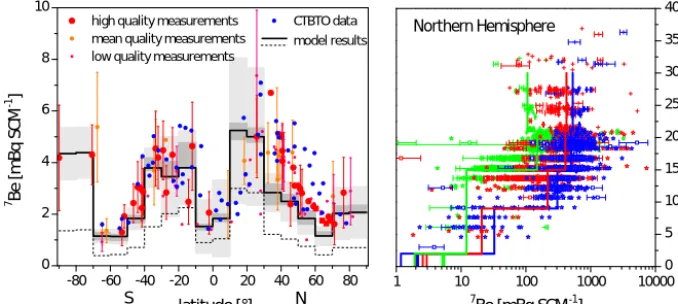
Figure 1 shows the comparison of mean7Be air activity concentration model results and measurements in latitudinal and vertical resolution. In the case of boundary layer obser-vations (Fig. 1, left), the measured reference values are mean values from long-term time series, while high-altitude7Be observations rely on punctual measurements within aircraft or balloon surveys and thus show stronger scattering (Fig. 1, right). Different model results based on either the Masarik and Beer (2009) or the Usoskin and Kovaltsov (2008) pro-duction rate calculations differ by a factor of 2.40 on av-erage (global avav-erage weighted with box sizes: 2.16). The differences show a latitudinal trend ranging from a factor of 1.7 (tropics) to 3.2 (polar latitudes) higher 7Be model re-sults in the case of the Usoskin and Kovaltsov (2008) pro-duction rate calculations. The model–measurement compar-ison reveals that the model quantitatively reproduces mean
7Be air activity concentrations in the global boundary layer if
the production rates from Usoskin and Kovaltsov (2008) are used. Model results based on the Masarik and Beer (2009) production rates clearly underestimate the observations by a factor of 2.4 on average. Having a look at the global distri-bution of atmospheric7Be, the model reproduces its main observed features: (i) a strong decrease from subtropical to mid- and high latitudes up to a factor of 5, (ii) a small7Be concentration in the tropics comparable to high (extra-polar) latitudes and, finally, (iii) a significant vertical gradient with
7Be air concentrations decreasing over 2 orders of
- 8 0 - 6 0 - 4 0 - 2 0 0 2 0 4 0 6 0 8 0
0
2
4
6
8
1 0
h i g h q u a l i t y m e a s u r e m e n t s C T B T O d a t a m e a n q u a l i t y m e a s u r e m e n t s
l o w q u a l i t y m e a s u r e m e n t s
N
l a t i t u d e [ ° ]
7 Be
[m
Bq
SC
M
-1 ]
S
m o d e l r e s u l t s
1 1 0 1 0 0 1 0 0 0 1 0 0 0 00
5
1 0 1 5 2 0 2 5 3 0 3 5 4 0
N o r t h e r n H e m i s p h e r e
al
tit
ud
e [
km
]
7B e [ m B q S C M - 1]
Figure 1. Model validation using global observations of the7Be activity air concentration (SCM is standard cubic meter). Left: model–
measurement comparison of mean7Be activity concentrations in boundary layer air. Different sizes and colors of measurements (circles and squares) denote different quality of long-term mean values: high quality (time series longer than 10 years, > 10 months of data per year on average), mean quality (time series longer than 3 years, > 9 months of data per year on average) and low quality (shorter time series and literature data without details on sampling time); circles denote mean values and squares represent median values. Note that all elevated sites (> 1000 m a.s.l.) except South Pole station at 90◦S are excluded. Blue symbols show unpublished data from the global CTBT monitoring system. These data allow for an independent model validation since sampling sites do not coincide with data used for model calibration. Model results are shown as black lines and grey shaded areas. Solid and dashed lines denote model results based on7Be production rate calculations by Usoskin and Kovaltsov (2008, solid line) and Masarik and Beer (2009, dashed line). The dark grey band indicates the model uncertainty from aerosol sink calibration. Light grey bars denote the standard deviation of the model results dominated by the seasonal cycle of the atmospheric concentrations. Model results encompass the mean of AD 1950–2000, whereas measurements represent various periods. Right: vertical distribution of7Be in the northern atmosphere according to US EML high-altitude sampling program data (symbols) and the GRACE model (lines) based on Usoskin and Kovaltsov (2008) production rates. Different colors denote different latitudinal bands according to the model resolution: polar (blue; 60–90◦N), mid-latitude (red; 30–60◦N) and tropical (green; 0–30◦N). Different symbols represent the three different high-altitude sampling programs: stars (STAR DUST), squares (AIRSTREAM) and crosses (ASHCAN). Data: Kolb (1992); Durana et al. (1996); Megumi et al. (2000); Ioannidou et al. (2005); Wershofen and Arnold (2005); Kulan et al. (2006); Kulan (2007); Feely et al. (1981, 1985, 1988); Larsen and Sanderson (1990, 1991); Larsen et al. (1995); Feely et al. (1967); Leifer and Juzdan (1986); Leifer (1992); Chae et al. (2011); Elsässer et al. (2011); Leppänen et al. (2012); Doering (2007), and references therein.
case of polar and mid-latitudes) of the simulated concen-trations in the respective northern free troposphere boxes. Different to the Southern Hemisphere, the model could thus have deficits in simulating the FT–BL vertical transport in the Northern Hemisphere. In the case of Antarctica, the7Be air activity concentration is significantly higher than in extra-polar high latitudes. Here, model results of the ice sheets are tuned to the mean observed 7Be air activity concentration (see Sect. 2.1.2) which precludes model validation. Compar-ing our model results of the 10Be air concentration (based on Kovaltsov and Usoskin (2010) production rates) to long-term observations from the coastal Antarctic Neumayer Sta-tion (Elsässer et al., 2011), our model only underestimates the measurements by 8 %. In the case of the Greenland ice sheet,10Be air concentration observations are restricted to 10 measurements covering the period June 1997–March 1998 (Stanzick, 2001). Here, model results exceed single month measurements by 30 % on average. However, due to the strong seasonal cycle (measured summer–winter ratio larger than 4) and the low data basis of 10 measurements, the10Be Greenland Summit model–measurement comparison is not very meaningful.
mod-els inability to reproduce the measured summer peak in the Greenland boundary layer7Be may thus originate from defi-cient simulation of210Pb (e.g., boundary layer transport from the Arctic basin to the Greenland ice sheet). Indeed, further model–measurement comparison of 7Be seasonal cycles at globally distributed sites (see in the Supplement Sect. S1, Fig. S5) reveals that the model performance is very good in mid- and polar latitudes (no 210Pb is involved in the model calibration). Major differences occur at low latitudes, only, where the model overestimates seasonal cycle amplitudes. Here, measurements in the tropics may be less representa-tive for 10◦ boxes due to large spatial differences in tropi-cal precipitation patterns (and thus lotropi-cal aerosol sinks, e.g., following monsoon patterns). On the multi-annual timescale, model–measurement comparison is difficult due to the over-all low signal-to-noise ratio of the 11-year production signal. Indeed, the extraction of this production signal from mea-sured time series is quite challenging (e.g., Koch and Mann, 1996; Aldahan et al., 2008; Elsässer et al., 2011). So far we eliminate the seasonal cycle of measurements and model re-sults by using a simple Gaussian smoothing filter to investi-gate the model’s ability to reproduce the production signal. Figure 2 reveals that the model clearly reproduces the cos-mogenic production signal inherent to the time series even if the shape of the solar cycle somewhat differs. In the case of the nearly 50-year time series at the PTB Braunschweig, the measurements show an increasing trend which is missing in the model data (see Fig. 2a). Excluding measurement ar-tifacts, possible explanations for this inconsistency are long-term climate effects (e.g., precipitation changes) which bias the atmospheric activity concentration and which are not considered in the observational-period model simulation.
In summary, the model validation shows that the model reproduces the climatology of7Be in the global atmosphere reasonably well. So far it is not possible to validate the model with10Be air concentration measurements since there are hardly any measurements available. However, given the model performance in terms of7Be, the model is likely also capable of simulating atmospheric10Be, since atmospheric concentrations of both (cosmogenic) radionuclides are gov-erned by similar atmospheric production and sinks.
2.1.4 The10Be production signal in polar areas
Having a well-calibrated and validated model of the global atmospheric10Be transport at hand, we investigated the ef-fect of atmospheric mixing on the10Be production signal in-herent to polar10Be. To do so, we ran the model under con-stant conditions of present atmospheric transport and mean solar activity (8=550 MV following Masarik and Beer, 1999) but modulated the geomagnetic dipole field. Figure 3 shows the simulated effect of geomagnetic changes on10Be in the polar atmosphere and on the global mean atmospheric
10Be concentration (i.e., the global atmospheric10Be
inven-tory). It is obvious that the10Be air concentration in the case
1 9 7 0 1 9 8 0 1 9 9 0 2 0 0 0 2 0 1 0
0
1
2
3
4
5
6
7
1 9 8 5 1 9 9 0 1 9 9 5 2 0 0 0 2 0 0 5 2 0 1 0
0
2
4
6
8
1 0
[m
Bq
SC
M
-1]
a ) 7B e i n B r a u n s c h w e i g
c ) 7B e a t G r e e n l a n d S u m m i t
[m
Bq
SC
M
-1 ]
b ) 7B e a t N e u m a y e r S t a t i o n
1 9 9 6 1 9 9 8 2 0 0 0 2 0 0 2 2 0 0 4 2 0 0 6 2 0 0 8 2 0 1 0 2 0 1 2
0
1
2
3
4
5
6
[m
Bq
SC
M
-1 ]
Figure 2. Comparison of measured (red circles) and modeled (black
lines)7Be air concentration time series (a) in Braunschweig, (b) at coastal Antarctica (Neumayer Station) and (c) at Greenland Sum-mit Station (near GISP2 drilling site). Model results (based on Usoskin and Kovaltsov (2008) production rate calculations) clearly match both features of the measurement time series, seasonal vari-ations and decadal production changes. Note that the Greenland and Antarctic model results are tuned to the overall mean7Be air concentration. In the case of the Braunschweig (52◦N) model– measurement comparison, the shown model results are 40–50◦N.
of the Greenland and Antarctic ice sheets is less sensitive to geomagnetic activity than the global mean10Be air concen-tration. However, this polar damping effect depends on the production calculations applied: in the case of Kovaltsov and Usoskin (2010) production rate data, the geomagnetic signal in Greenland is up to 50 % lower than the global mean sig-nal. Usage of the Masarik and Beer (2009) calculations only results in up to 22 % lower modulation of Greenland10Be. Certainly, this discrepancy is based on different geomagnetic modulation of the global mean10Be inventory: both produc-tion rate calculaproduc-tions differ in their latitudinal shape of the
10Be production (i.e., their dependency of10Be production
- 7 5 - 5 0 - 2 5 0 2 5 5 0 7 5 1 0 0 - 5 0
- 2 5
0
2 5 5 0 7 5 1 0 0 1 2 5
A n t a r c t i c I c e S h e e t
g l o b a l m e a n
b ) M a s a r i k a n d B e e r ( 2 0 0 9 ) p r o d u c t i o n r a t e c a l c u l a t i o n s
A n t a r c t i c I c e S h e e t
G r e e n l a n d I c e S h e e t
ch
an
ge
fr
om
p
re
se
nt
10Be
air
co
nc
en
tra
tio
n
[%
]
c h a n g e f r o m p r e s e n t g e o m a g n e t i c d i p o l e f i e l d [ % ]
g l o b a l m e a n
a ) K o v a l t s o v a n d U s o s k i n ( 2 0 1 0 ) p r o d u c t i o n r a t e c a l c u l a t i o n s
- 7 5 - 5 0 - 2 5 0 2 5 5 0 7 5 1 0 0- 5 0
- 2 5
0
2 5 5 0 7 5 1 0 0 1 2 5
G r e e n l a n d I c e S h e e t chan
ge
fr
om
p
re
se
nt
10 Be
air
co
nc
en
tra
tio
n
[%
]
Figure 3. Modeled influence of the geomagnetic dipole field changes on atmospheric10Be illustrating the effect of atmospheric mixing.
The left and right panel differ in the production rate calculations applied in the model simulations; (a) Kovaltsov and Usoskin (2010) or
(b) Masarik and Beer (2009). Different lines show the global mean10Be air concentration (black) and local10Be air concentration on the
Greenland (light blue) and Antarctic (deep blue) ice sheet. Solar activity is held constant at 550 MV. Note that the uncertainty of aerosol sink calibration (shown in Fig. 1) does not significantly influence the above results.
rates. The reason for this finding is that polar areas do not re-ceive a globally mixed production signal. This atmospheric transport effect makes polar ice core10Be-based reconstruc-tions of past geomagnetic activity less sensitive to the choice of10Be production rate calculations. This however does not hold for solar-activity-based production changes. Here, our model results show larger solar modulation of the polar10Be air concentration compared to the global mean (not shown). However, in comparison to the polar damping in the case of geomagnetic variations, this polar enhancement effect is less pronounced (9–16 and 12–17 % in the case of the Kovaltsov and Usoskin (2010) and Masarik and Beer (2009) production rates). In summary, our results reveal that polar latitudes do not receive a globally well-mixed atmospheric10Be produc-tion signal. In recent years, two GCM studies investigated the atmospheric footprint of the polar 10Be deposition flux though achieved inconsistent results. Assuming that the po-lar 10Be deposition is controlled by polar boundary layer
10Be air concentration, our finding contradicts to GCM
re-sults from Heikkilä et al. (2009) (based on ECHAM5-HAM) but is in line with the results of Field et al. (2006) (using the GISS ModelE). The latter authors report on 20 % reduc-tion of the geomagnetic modulareduc-tion of polar10Be (based on
Masarik and Beer (1999) production rates and in the case of a geomagnetic field decreased by 25 %). Using Masarik and Beer (2009) production rate calculations, our Green-land model simulations quantitatively confirm this result: 20– 22 % lower geomagnetic modulation within the total range of analyzed global geomagnetic field changes.
2.2 Local air–firn transfer
Different and complex processes contribute to the hand over of atmospheric10Be into polar firn (see, e.g., Slinn, 1977), which still lack proper understanding. We therefore refrain
from deploying a full physical process model but use a rather basic, measurement-calibrated air–firn transfer model ap-proach to simulate the transfer of10Be from the polar bound-ary layer air into firn. In doing so we use observed spatial trends in polar10Be ice concentration to investigate its cli-mate modulation. Across both the Greenland and the Antarc-tic ice sheets, climate conditions show large spatial gradients essentially between coastal areas and the remote interior. The ice sheets rise closely to the coast and mount up to 3 and 4 km (in the case of Greenland and Antarctica) entailing colder and dryer conditions at the polar plateaus. The observed dif-ference in mean snow accumulation rates between coastal sites and the interior of the ice sheet amounts up to a fac-tor of > 25 (Law Dome:>60 cm year−1, Smith et al., 2000; Vostok: 2.3 cm year−1, Pourchet et al., 2003). These differ-ent climate conditions coincide with major differences in the mean10Be ice concentration of more than a factor of 8 (see Fig. 4). On the other hand, mean radionuclide air concen-trations above the snowpack do not show large differences (e.g., Elsässer et al., 2011). The spatial gradient in the10Be ice concentration is thus governed by the processes deliver-ing 10Be from air to firn. Investigating this modulation of the10Be ice concentration by spatial change in local climate
conditions therefore allows for investigation of the air–firn transfer and its climate variability.
2.2.1 Formulation of the basic air–firn transfer model
inter-val (1t=t1−t0) may be expressed as
c1tice=
Rt1
t0[Jdry+Jwet]dt
Rt1
t0Adt
. (1)
The10Be dry deposition flux depends on the10Be surface air concentration and the dry deposition velocity (vdry). It
comprises all deposition processes which are not related to precipitation. The wet deposition is the concentration of10Be in fresh snow times the precipitation rate (P). Assuming that both, the dry and wet deposition fractions are controlled by the same air mass, we may substitute the snow concentration using the scavenging ratio (ε– volume-based ratio between radionuclide concentration in snow and air) and get
c1tice= Rt1
t0[vdry·cair+P·csnow]dt
Rt1
t0Adt
= Rt1
t0[vdry+P·ε] ·cairdt
Rt1
t0Adt
. (2)
On a well-chosen, climatological timescale we may as-sume the dry deposition velocity, the precipitation rate and the scavenging ratio as being a characteristic constant and get a first-order approximation of “climatologically averaged” terms
cice=
vdry+P·ε
A
!
·cair. (3)
The relation between precipitation rate and net accumu-lation rate depends on wind drift and evapo-sublimation. In polar areas, it is reasonable to assume the relation as being constant on a climatological timescale. The precipitation and net accumulation ratio may then be included into a modified scavenging ratio parameterε∗. Since this parameter eludes a straightforward physical interpretation, we refrain from ex-plicitly discriminating betweenεandε∗and get
cice=
v
dry
A
+ε
·cair. (4)
Following this basic air–firn transfer model, three main parameters govern the hand over of 10Be from air to firn: the accumulation rate (A), the dry deposition velocity (vdry)
and the scavenging ratio (ε). While vdry and ε cannot be
measured directly, the relation between the measured mean
10Be ice concentration and mean observed snow
accumula-tion rates can be investigated in a straightforward way. To do so, we compile published mean 10Be ice concentrations from different Antarctic sampling sites in addition to eight unpublished 10Be firn core time series (Neumayer Hinter-land, Kohnen Station, Berkner Island and Dome C). Fig-ure 4a shows the compiled 10Be ice concentration plotted against inverse mean snow accumulation rates at respective sites. Due to the involvement of different AMS laborato-ries in the 10Be measurements, we recalibrated the differ-ent data using results from Nishiizumi et al. (2007) and Ku-bik and Christl (2010). Furthermore, we correct the effect
of different temporal coverage and thus production variabil-ity of the10Be measurements (Fig. 4b; see Sect. S2 for de-tails). The latter correction imposes revisions between−4.1 and 12.6 % to single data points. Eventually, Fig. 4b reveals that the mean10Be ice concentration at different Antarctic sites is well correlated to the inverse accumulation rate (cor-relation coefficient: 0.97). Hence, we conclude that spatial variation in the mean 10Be ice concentration is driven by spatial accumulation changes at first order. The major dif-ferences between meteorological conditions at coastal and interior Antarctica seem to have less influence on the dry deposition velocity or aerosol scavenging. This finding al-lows for estimating the two missing parameters (vdryandε)
of the basic model (Eq. 4) by investigating the relation be-tween measured10Be ice concentration and corresponding snow accumulation rates.
2.2.2 Determination of model parameters
10Be measurements within Greenland and Antarctic traverse
surveys allow for more detailed investigations of the air–firn transfer processes. In comparison to the compilation of10Be literature data (Fig. 4), this approach allows for further re-ducing some uncertainty: (i) Measurements within each sur-vey are conducted by only one AMS laboratory (see, e.g., Merchel et al., 2012 for comparability of different AMS fa-cilities), (ii) all samples analyzed for the mean10Be ice con-centrations broadly cover the same period of time and (iii) es-pecially in the case of Antarctica, the spatial scale of single traverses is comparatively small (i.e., a few 100 km). It is thus very likely that all sampling sites are affected by comparable atmospheric transport conditions.
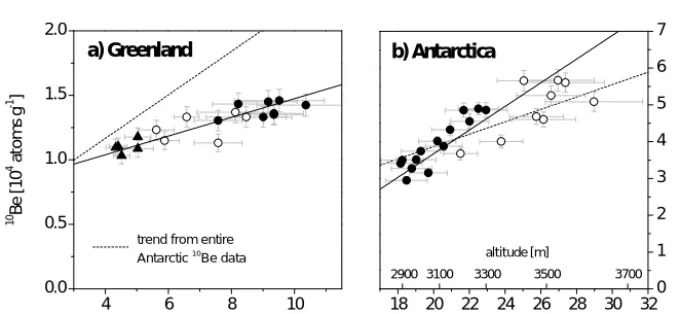
Surveys in Greenland and Antarctica were accomplished in cooperation with the Alfred Wegener Institute dur-ing 1990–1992 (Expedition Glaciologique Internationale au Groenland, EGIG), 1993–1995 (North Greenland Traverse, NGT) and 2006 (EDML upstream traverse). In addition, fur-ther snow-pit samples from the Antarctic Japanese–Swedish (JASE) traverse in 2007–2008 were analyzed for mean10Be ice concentrations. Details on the traverses and the 10Be measurements are given in the Supplement (Sects. S2.3 and S.2.4). Figure 5 presents the results separated into Green-land and Antarctic measurements and compared to the linear trend of (mostly published) Antarctic-wide data (as shown in Fig. 4). Our measurements clearly confirm the finding of a linear relation between10Be ice concentration and the inverse accumulation rate. However, in both cases, the lin-ear trend differs from the compilation of10Be measurements from the entire Antarctica: in the case of Greenland traverses, the slope of the linear fit falls below the Antarctic literature by a factor of 2.3. The10Be measurements within the Antarc-tic traverses reveal a factor of 1.9 stronger trend.
0 1 0 2 0 3 0 4 0 5 0
0
2
4
6
8
1 0
D M L
b )
T a y l o r D o m e S o u t h
P o l e S i p l e D o m e
L a w D o m eB e r k n e r I s l a n d K o h n e n
D o m e C V o s t o k
10 Be
[1
0
4 at
om
s g
-1 ]
D o m e F
a )
0 1 0 2 0 3 0 4 0 5 0 0
2
4
6
8
1 0
N e u m a y e r h i n t e r l a n d
D o m e F
L a w D o m e S i p l e D o m e
B e r k n e r I s l a n d K o h n e n
D o m e C V o s t o k
10 Be
[1
0
4 at
om
s g
-1 ]
i n v e r s e s n o w a c c u m u l a t i o n r a t e [ y r m - 1]
Figure 4. Mean10Be ice concentrations from various sites in Antarctica plotted against corresponding (inverse) snow accumulation rates
(given in water equivalent). Filled dots refer to published data while open circles represent unpublished data. (a) Originally published values without any correction. Error bars denote the standard deviation of the respective time series. (b) Mean10Be concentrations corrected for different time coverage and AMS measurement standards (see Sect. 2.2 for details). Here, error bars show an average AMS uncertainty of 5 %. Note that, different to (a),10Be data sets which lack information on the AMS calibration standard used for measurements are disregarded. The straight line denotes a linear fit to the data and the dark grey shaded area depicts the formal fitting error. Light grey shaded area is based on 25 % higher and lower slope (andyintercept) and covers all data points (except two outliers: 12 % of total number). Data: Raisbeck et al. (1990); Steig (1996); Aldahan et al. (1998); Smith et al. (2000); Nishiizumi and Finkel (2007); Horiuchi et al. (2008); Baroni et al. (2011); Pedro et al. (2012); Steinhilber et al. (2012). Further accumulation rate data: Jouzel et al. (1979); Sommer et al. (2000); Hamilton (2002); Pourchet et al. (2003); Oerter et al. (2004); Fernandoy et al. (2010).
4 6 8 1 0
0 . 0 0 . 5 1 . 0 1 . 5 2 . 0
t r e n d f r o m e n t i r e A n t a r c t i c 1 0
B e d a t a
10 Be
[1
0
4 at
om
s g
-1 ]
a ) G r e e n l a n d
1 8 2 0 2 2 2 4 2 6 2 8 3 0 3 2 0
1
2
3
4
5
6
7
10 Be
[1
0
4 at
om
s g
-1 ] b ) A n t a r c t i c a
i n v e r s e s n o w a c c u m u l a t i o n r a t e [ y r m - 1]
2 9 0 0 3 1 0 0 3 3 0 0 3 5 0 0 3 7 0 0 a l t i t u d e [ m ]
Figure 5. Spatial distribution of mean10Be firn concentrations measured within (a) Greenland and (b) Antarctic traverses. While solid lines
denote linear fits to the above measurements, dashed lines depict the linear fit to Antarctic-wide data shown in Fig. 4. In both cases, Greenland and Antarctica, different symbols denote different traverse surveys: (a) NGT west (•), NGT east (N), EGIG east (◦). (b) Kohnen upstream (•), JASE (◦) (see Sects. 2.3 and 2.4 for details).
the case of Antarctica, Elsässer et al. (2011) reported on 25 years of atmospheric 10Be measurements at the coastal Neumayer station and found a mean air concentration of 4.6×10⁴atoms SCM−1(standard cubic meter). In the case of Greenland, 10Be air concentrations have to be deduced from 16 years of7Be measurements at the Greenland Sum-mit Station (see Fig. 2) using a constant 10Be/7Be ra-tio. The latter is based on 10 months of 10Be measuments at Greenland Summit Station (Stanzick, 2001) re-sulting in a mean Greenland Summit 10Be air
concentra-tion of (2.4±0.4)×104atoms SCM−1(uncertainty from7Be and10Be/7Be-based estimates). The difference in the mean
10Be air concentration at Antarctic Neumayer and Greenland
Summit sites is in line with the atmospheric7Be measure-ments at both sites which differ by a factor of 1.8 on av-erage. Inserting these10Be air concentrations, our observed
10Be ice concentrations and corresponding snow
10Be dry deposition velocities of (0.10±0.02) cm s−1 and
(0.22±0.03) cm s−1 for Greenland and Antarctica,
respec-tively. Thus, at first glance, our10Be measurements point to a stronger dry deposition velocity in Antarctica which may be caused by different glacio-meteorological conditions (i.e., non-precipitation-related processes like water vapor conden-sation on, and sublimation from the the snow surface). How-ever, using the trend from the compilation of10Be measure-ments over the entire Antarctica (Fig. 4) within the model, the resulting dry deposition of (0.116±0.003) cm s−1meets the Greenland results surprisingly well. Different reasons may account for the mismatch between the local Antarctic traverses around Kohnen Station and the entire Antarctic data compilation. At first the assumption of a constant 10Be air concentration over the entire Antarctica is a rough oversim-plification and regional trends in atmospheric10Be could af-fect the results of the large-scale data compilation. On the other hand, the determination of mean accumulation rates in dry Antarctic conditions is challenging (see Sect. S2.4) and the Antarctic-wide data compilation thus allows for a more robust estimation of accumulation rate trends. Within this study we focus on Greenland model results and use an over-all dry deposition velocity of 0.1 cm s−1. In the case of model results for Antarctica, both ongoing measurements of atmo-spheric10Be at the high Antarctic plateau and ongoing exten-sion of10Be ice concentration measurements to very low ac-cumulation sites will provide further constraints on the model parameters. The second decisive parameter for the10Be air– firn transfer is the volume-based ratio between10Be air and firn concentration (scavenging ratio). Applying Eq. (4) to the spatial 10Be trends gives a ratio of (3.1±0.6)×105 [atoms m−air3/atoms m−3
snow] for Greenland which corresponds
to a 10Be concentration of (7.5±0.7)×103[atom g−1] in fresh fallen snow. Here, the model applied to Antarctic liter-ature data gives a factor of 2.8 lower scavenging ratio. Again the generally dryer and colder conditions may be responsible for this difference.
2.2.3 Dry versus wet deposition at Greenland Summit
The site-specific ratio of dry versus wet deposition of10Be is a valuable parameter for the interpretation of10Be ice core records. Generally speaking, in case of dominating wet depo-sition processes, the10Be ice concentration is less influenced by accumulation rate changes making the 10Be ice concen-tration a primary reference for atmospheric10Be production changes (see, e.g., the detailed discussion in Alley et al., 1995). On the other hand, dominating dry deposition impli-cates larger influence of snow accumulation variability. Here, the interpretation of the 10Be deposition flux (derived from
10Be ice core records) in terms of cosmogenic production
changes is common practice (e.g., Muscheler et al., 2004, 2005). Our air–firn transfer model results indicate that wet deposition processes dominate the Greenland Summit10Be ice concentration under present conditions (mean snow
accu-mulation rate at GRIP drilling site: 0.21 m yr−1water
equiv-alent; Johnsen et al., 1992) and dry deposition only accounts for 32 % of the total10Be deposition. Assuming an overall mean Greenland precipitation rate of 0.3 m yr−1(Bales et al., 2001), this value is slightly lower for the entire Greenland (24 %) and the10Be sink in the Greenland ice sheet model box (see Sect. 2.1). Using210Pb instead of10Be measure-ments results in a similar Greenland ice sheet dry to total deposition ratio of 30 % (Stanzick, 2001). It is worth men-tioning that this figure holds as well for the (sub-micron) non-sea-salt sulfate distribution in central Greenland inves-tigated by Fischer and Wagenbach (1996). Using the same deposition model approach they arrived at a dry deposition flux fraction of 37 % for this species which was consistent with the direct observations reported by Bergin et al. (1995) from Summit.
Global circulation model results (Field et al., 2006; Heikkilä et al., 2008a) report a larger impact of wet depo-sition in the case of Greenland (i.e., dry depodepo-sition less than 10 %). So far, this mismatch remains unexplained. However, regarding the GCM results from Heikkilä et al. (2008a), over-estimated wet deposition might contribute to their signifi-cantly underestimated Antarctic7Be activity air concentra-tion. Finally, in terms of interpreting10Be ice core records, the ratio of dry to total deposition flux is most likely not con-stant under climate change. Investigating temporal changes in10Be deposition at Greenland Summit, Alley et al. (1995) found that any variations in the dry deposition velocity and scavenging ratio have been small. We may thus assume linear scaling of wet deposition with accumulation rates to investi-gate the effect of climate change on the ratio of dry to total deposition. Using reconstructed variations of the GRIP snow accumulation rate (see also Fig. 7a) as model input we find that the10Be air–firn transfer at Greenland Summit is domi-nated by dry deposition (ratio of dry to total deposition up to 65 %) during the last glacial stadials.
Alley et al. (1995) regressed10Be (among other aerosol species) from the Summit GISP2 core versus accumula-tion rate (using the same deposiaccumula-tion model approach as the present study). The authors inferred the relative change in the atmospheric10Be load between late glacial (cold) stadials and (warm) interstadials. Here, the temporal changes of the deposition regime climatology have been deployed instead of spatial changes as done in the present study. Their finding limits the respective cold/warm10Be ratio to less than 1.5 with the most likely ratio around 1.2.
2.3 Looking into the past: model simulations on the
glacial–interglacial timescale
depen-atmosphere
solar activity, geomagnetic field, precipitation changes
air-firn
transfer
10Be air
concentration
snow accumulation at individual site
atmosphere
transfer
air-firn
10Be air
concentration
10Be ice concentration
at individual site
10Be large scale
deposition flux
Figure 6. Sketch of our basic model approach to simulate 10Be
ice core records on the glacial–interglacial timescale. The model setup of the atmosphere is presented in Sect. 2.1, whereas the air– firn transfer model is put forward in Sect. 2.2. Model input records are discussed in Sect. 2.3.
dency of the model results. Both, variations of10Be produc-tion and changes in climate condiproduc-tions have to be taken into account and will be addressed subsequently. The final model setup for the investigation of10Be ice core records is sum-marized in a basic sketch shown in Fig. 6.
2.3.1 Production variability
A fundamental process influencing the temporal variability of ice core 10Be is its atmospheric production rate. Basi-cally, solar activity, changes in the geomagnetic field strength as well as variations in the galactic cosmic ray flux mod-ulate the atmospheric production of 10Be. However, only geomagnetic variations have been clearly proven to impose multi-millennial variations on the production rate of cos-mogenic radionuclides. Therefore, focusing on the glacial– interglacial timescale, we restrict changes of the 10Be pro-duction to variations in the geomagnetic dipole field. We choose the high-resolution geomagnetic reconstruction from Laj et al. (2004) which is based on a selection of 24 high-accumulation marine sediment records (GLOPIS-75). The record is converted from the GISP2 timescale to the most up-to-date Greenland ice-core chronology (GICC05modelext timescale), by using partly unpublished match points be-tween the NorthGRIP, GRIP and GISP2 ice cores (Seierstad et al., 2014) (see Fig. 7b and Sect. S3.1). Since geomagnetic modulation of polar10Be is not very sensitive to the choice of different production rate calculations (see Sect. 2.1.4), we use the production rate calculations of Kovaltsov and Usoskin (2010) throughout. Solar activity is kept constant at a mean value of 550 MV (Masarik and Beer, 1999). In-deed, solar activity might also show variation on timescales longer than the well-known multi-centennial period. How-ever, (10Be-independent) 14C-based reconstructions are so far restricted to the Holocene period. Here, differences in
10Be- and14C-based reconstructions leave the magnitude of
multi-millennial variations of solar activity subject to debate (Vonmoos et al., 2006).
2.3.2 Climate variability
It is important to highlight that our model approach essen-tially differs from global climate model attempts and does not allow for implicit climate modulation of atmospheric10Be by, e.g., varying the atmospheric concentration of greenhouse gases. However, we may explicitly vary processes which have been proven to (i) influence the10Be ice concentration and (ii) vary on the glacial–interglacial timescale. So far, we restrict climate modulation to precipitation/snow accumula-tion changes which are comparatively well known. Precipi-tation governs both, the tropospheric residence time of10Be (i.e., the10Be deposition; Heikkilä and Smith, 2013) and the local10Be air–firn transfer (Stanzick, 2001). Recent GCM model results by Heikkilä et al. (2013) indicate that changes in the 10Be deposition are also consistent with precipita-tion changes under different climate condiprecipita-tions. However, the authors find additional atmospheric circulation changes influencing the10Be air concentration (mainly in higher at-mospheric layers). Future applications of the model setup presented here may easily include further processes of cli-mate variability (as, e.g., modulation of atmospheric air mass transport). However, for this study, changes in the atmo-spheric circulation or air–firn parameterization (i.e., dry de-position velocity and aerosol scavenging) are not taken into account. We are well aware that this simplistic approach is a rough oversimplification. However, sensitivity studies on at-mospheric transport and deposition indicate that present-day polar boundary layer10Be is quite robust against global-scale circulation changes (Elsässer, 2013). On the contrary, these studies indicate that polar boundary layer10Be is very sen-sitive to local polar air mass transport (i.e., boundary layer– free troposphere coupling). This is reasonable given the ra-dionuclide concentration in the (polar) free troposphere ex-ceeding common (polar) boundary layer concentrations by an order of magnitude (see Fig. 1 for7Be). Still, processes of ice sheet boundary layer atmospheric transport are not under-stood sufficiently and global circulation models have issues with reproducing polar7Be sufficiently well. We are thus not sure if usage of complex climate models would significantly improve simulations of local conditions on the ice sheets.
sum-0 . sum-0 0 . 1 0 . 2 0 . 3
c ) m o d e l r e s u l t s :1 0B e i c e
c o n c e n t r a t i o n
b ) m o d e l i n p u t : g e o m a g n e t i c d i p o l e f i e l d
[m
ye
ar
-1 ]
G R I P G I S P 2 m e a s u r e m e n t s
m o d e l
a ) m o d e l i n p u t : G R I P a c c u m u l a t i o n r a t e
0
5
1 0 1 5 2 0
V
AD
M
[1
0
22 A
m
2 ]
0
2
4
6
8
[1
0
4 at
om
s g
-1 ]
0
2
4
6
[r
ela
tiv
e t
o
H
ol
oc
en
e]
d ) m o d e l r e s u l t s : r e l a t i v e t o H o l o c e n e
e ) m o d e l - m e a s u r e m e n t s d i f f e r e n c e
7 0
6 0
5 0
4 0
3 0
2 0
1 0
0
- 5 0
0
5 0 1 0 0 1 5 0
m
od
el-m
ea
su
re
m
en
ts
d
iff
er
en
ce
o
f d
) [
%]
m
od
el-m
ea
su
re
m
en
ts
d
iff
er
en
ce
o
f c
) [
%]
a g e [ k y r b 2 k ]
- 5 00
5 0 1 0 0
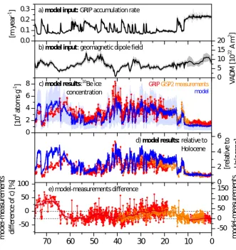
Figure 7. Model results of the10Be ice concentration at Greenland Summit compared to respective ice core measurements. (a) and (b) show
the model input data driving the temporal variation of the model results: GRIP accumulation and geomagnetic dipole field strength (Laj et al., 2004) both on the GICC05modelext timescale (see text for details). (c) shows the10Be model results (blue) compared to GRIP (red dots; Yiou et al.,1997; Wagner et al., 2001a; Muscheler et al., 2004) and GISP2 (orange dots; Finkel and Nishiizumi, 1997) measurements. The blue band denotes the original model results including the seasonal cycle. Thick blue lines show yearly mean model results. (d) shows model results and measurements normalized to the Holocene period. Model–measurement differences of (c) and (d) are shown in (e) relative to measurements. Here, thick lines denote Gaussian smoothing which dampens 2000-year oscillations to 0.1 %.
marizing common findings, model inter-comparison projects report on glacial drying being the largest over the ice sheets and sea ice (Braconnot et al., 2007). Ice-core-based recon-structions of precipitation rates may thus give an upper limit to glacial–interglacial differences. For our model study, we use a revised version of the GRIP snow accumulation rate (Fig. 7a) based on the GICC05modelext timescale (see Sect. S3.1). We use two different scenarios for adopting the ice-core-based precipitation changes to the hemispheric pre-cipitation pattern: (i) Prepre-cipitation in the Greenland ice sheet box modulated by relative changes of the GRIP accumulation rate, but constant precipitation rates in the residual northern hemispheric boxes. (ii) precipitation in the entire high lat-itudes boxes (60–90◦N) modulated by relative changes of the GRIP accumulation rate but constant precipitation rates in mid- and low latitudinal boxes (0–60◦N). However,10Be
3 Results for Greenland Summit
Finally, we present forward model results for the Green-land Summit10Be ice concentration covering the last 75 kyr. Since the GRIP and GISP210Be ice core profiles are widely used in different studies (e.g., Muscheler et al., 2004, 2005; Köhler et al., 2006), model–measurement comparisons of the two Greenland Summit ice core records is especially infor-mative. However, for future investigations, model simula-tions can be easily expanded for different sampling sites in Greenland and Antarctica, if site-specific changes of snow accumulation are known sufficiently well.
3.1 Results
Modeled Greenland Summit10Be ice concentration time se-ries is shown in Fig. 7 together with the measured profiles from the GRIP and GISP2 ice cores (Finkel and Nishiizumi, 1997; Yiou et al., 1997; Wagner et al., 2001a; Muscheler et al., 2004) and the time-dependent model input data. The mea-surements have been corrected for10Be decay (3.8 % at most for the last 75 kyr), revised AMS calibration (Nishiizumi et al., 2007) and sample processing effects (see Sect. S3.2 for details). Neither the GRIP nor the GISP2 10Be measure-ments cover the observational period. However, comparing our model results to firn core10Be measurements from the GRIP drilling site, we find that the model only underesti-mates the recent10Be ice concentration by 4 % (Heikkilä et al., 2008b) and 6 % (Stanzick, 1996) (firn core accumulation rates taken from respective studies and solar activity taken from Usoskin et al., 2011). Due to lack of measurements, it is not possible to directly validate the simulated10Be air concentration at Greenland Summit (see Sect. 2.1.3). How-ever, we may specify the model–measurement deviation of the air–firn transfer model (which is the difference of ob-served 10Be ice concentration at a single site to the over-all linear fit in Fig. 5). In the case of both Greenland Sum-mit firn cores, the overall model–measurement divergence is dominated by this air–firn transfer model divergence (4 and 5 %) which points to a good overall performance of the at-mospheric model in reproducing the10Be air concentration in Greenland. In the case of the entire Holocene period, abso-lute model–measurement differences are larger (see Fig. 7c and e) with the model underestimating observed 10Be ice concentrations by 27 % (mean GRIP; median: 27 %; inter-quartile range: 12 %) and 24 % (mean GISP2; median: 24 %; inter-quartile range: 14 %).
Focusing on glacial–interglacial changes of the10Be ice concentration we compare our model results to the observed ice core records on a normalized scale. In doing so we use the major part of the Holocene period where GRIP 10Be mea-surements are available (9361–355 yr b2k) as reference and divide the time series by this “Holocene mean”. In the case of the GISP2 record, measurements do not cover this whole period and we use the GRIP Holocene 10Be ice
concentra-tion for normalizaconcentra-tion. Figure 7d reveals that the model cap-tures both dominant feacap-tures of the measured10Be ice core records: (i) a factor of 2–3 rise in the 10Be ice concentra-tion from Holocene to glacial periods and (ii) the millennial-scale variability during the last glacial period related to Dansgaard–Oeschger events. During the glacial period, the model (normalized to the Holocene) overestimates the GRIP and GISP2 data by 19 % (mean: 22 %, inter-quartile range: 39 %) on average. However, model–measurement residu-als are not randomly distributed around a constant offset but show some significant low-frequency oscillations (see Fig. 7e, right axis). The most prominent model–measurement difference occurs during the (62–75 kyr) b2k period, where the model (normalized to the Holocene) overestimates mea-sured10Be ice concentrations by 65 % on average (median: 74 %, interquartile range: 61 %). Here, smoothed model– measurement differences come up to 87 % of the observed mean Holocene10Be ice concentration. Moreover, the model significantly overestimates the observations in 12–37 kyr b2k (average: 31 % GRIP, 20 % GISP2) and 43–52 kyr b2k (av-erage: 15 % GRIP). On the other hand, the mean model– measurement differences are low during 37–43 and 52– 62 kyr b2k.
3.2 Discussion
Given the large variations inherent to the 10Be ice con-centration our basic model reproduces the largest part of the observed 10Be ice core records. It is of major interest that the model–measurement differences do not show a con-stant offset over the entire glacial period. In addition, cor-relation analysis with the GRIP δ18O record (primary ref-erence for climate variability; Johnsen et al., 1997) reveals that the model accounts for the major part of climate mod-ulation: while the measured10Be ice concentration shows a significant negative correlation (GRIP:r= −0.75; GISP2: r= −0.90), model–measurement differences (as shown in Fig. 7e) are less correlated to the stable isotopes record (GRIP: r= −0.38; GISP2: r= −0.43). This finding does also hold for the glacial period, indicating that the model explains a major fraction of fast glacial climate variations (related to Dansgaard–Oeschger events). However, the multi-millennial trends in the model–measurement differences (up to 87 % of the Holocene mean) call for a detailed discussion of their likely origin. Deficient model input records as well as unconsidered climate variations could basically account for this model–measurement mismatch.
0
1
2
3
4
5
6
b )
c l i m a t e f o r c i n g o n l y
a i r f i r n t r a n s f e r o n l y p r o d u c t i o n f o r c i n g o n l y
10 Be
ic
e
co
nc
en
tra
tio
n
[re
lat
ive
to
H
ol
oc
en
e] m o d e l r e s u l t s : f u l l f o r c i n g
c l i m a t e f o r c i n g : a t m o s p h e r i c s i n k f o r c i n g o n l y
a )
7 0 6 0 5 0 4 0 3 0 2 0 1 0 0 0 . 7 5
1 . 0 0 1 . 2 5 1 . 5 0 1 . 7 5 2 . 0 0 2 . 2 5 2 . 5 0
10 Be
ic
e
co
nc
en
tra
tio
n
[r
el
at
ive
to
H
ol
oc
en
e]
a g e [ k y r b 2 k ]
Figure 8. Sensitivity of Greenland Summit10Be ice concentration model results with respect to different influencing processes. (a) Model
results using constant geomagnetic activity (climate forcing only, orange) compared to model results with constant precipitation/snow accu-mulation rate (production forcing only, black) and full forcing (blue). (b) Breakdown of climate modulation into air–firn transfer (red) and atmospheric sink strength (light red).
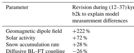
of the overall Holocene mean10Be ice concentration. Apart from that, the geomagnetic modulation is generally lower than 36 % which is comparable to the model–measurement differences. Indeed, focusing on the (12–37) kyr b2k period, the geomagnetic dipole record applied in the model simu-lations (GLOPIS75, Laj et al., 2004) would need average revision by +222 % to adapt the (normalized to Holocene) model results to the measurements. This would result in a geomagnetic dipole moment which would exceed the mean Holocene value. It is thus very unlikely that geomagnetic changes account for a major part of the model–measurement differences. The atmospheric production of10Be could how-ever also hold multi-millennial modulation due to solar activ-ity. Though not varied in the model simulations, long-term trends in solar activity could thus contribute to the model– measurement differences (see, e.g., Vonmoos et al. (2006) for Holocene multi-millennial variations reconstructed from14C and10Be). Indeed our model results show that the polar10Be ice concentration is more sensitive to solar activity than the global mean10Be air concentration (see Sect. 2.1.4). How-ever, regarding the (12–37) kyr b2k period, the (so far con-stant) solar activity would require average increase by+72 % to explain the (relative to Holocene) model–measurement differences. We may thus conclude that production changes are not responsible for a large share of the model shortcom-ings. This does not hold for climate modulation of the10Be ice concentration. Here, precipitation and snow accumula-tion changes modulate the simulated10Be ice concentration up to 400 % (Fig. 8a). The applied GRIP snow accumula-tion record would require much less revision to account for
dif-Table 1. Required revision of model input records to account for
the (normalized to Holocene) model–measurement differences dur-ing (12–37) kyr b2k (30 % of the observed Holocene mean, com-bined GRIP–GISP2 record). Note that, different to the geomagnetic dipole strength and the Greenland snow accumulation rate, the orig-inal model input parameters for solar activity and the diffusive BL– FT do not vary on a multi-annual scale.
Parameter Revision during (12–37) kyr
b2k to explain model measurement differences
Geomagnetic dipole field +222 %
Solar activity +72 %
Snow accumulation rate +28 % Diffusive BL–FT coupling −26 %
ferences during (12–37) kyr b2k could be explained by an average reduction of the diffusive boundary layer–free tro-posphere coupling by only 26 %. It is thus very likely that model–measurement differences are related to climate vari-ability (see Table 1 for a summary of the sensitivity studies). Adequate knowledge of changes in10Be atmospheric trans-port and deposition is thus a fundamental requirement for
10Be ice-core-based reconstruction of geomagnetic and solar
activity.
4 Summary and outlook
We present a climatological model approach of the10Be ice concentration which allows for the first quantitative (sub-annual-resolution) simulations up to the glacial–interglacial timescale. The model thus satisfies the demand for an easy-to-use tool to support the interpretation of10Be ice core mea-surements on long timescales. In specifically configuring the model setup for ice core 10Be, we coupled a (coarse grid) model of the global atmosphere to a basic, measurement-supported air–firn transfer model. In addition to polar mea-surements of 10Be, comprehensive observational data of different (cosmogenic, anthropogenic and terrigenic) short-lived aerosol-borne radionuclides on the global and polar scale have been applied for model calibration and validation. Investigating the production signal of 10Be in polar ar-eas, our model results show that 10Be is not well mixed in the global atmosphere. In comparison to the global mean atmospheric 10Be concentration, polar 10Be is less modu-lated by changes of the geomagnetic dipole field (but more sensitive to solar activity). In the case of Greenland, the amount of this polar damping of the geomagnetic modula-tion of10Be comes up to 50 %, but significantly depends on the production rate calculations applied. Indeed, calculations based eather on the Masarik and Beer (2009) or on the Ko-valtsov and Usoskin (2010) production rates reveal signifi-cantly different geomagnetic modulation of the global mean
10Be air concentration. However, model results using the
dif-ferent production rate calculations coincide in the geomag-netic modulation of10Be at polar latitudes. Reconstructions of past geomagnetic activity based on ice core10Be are there-fore not very sensitive to the production rate calculations ap-plied. However, this does not hold for solar-activity-induced changes of polar10Be.
On the glacial–interglacial timescale, observed Greenland
10Be ice core records show large variation of up to 400 %
from the overall Holocene mean. Applying the model to sim-ulate the Greenland Summit (GRIP and GISP2)10Be ice core records, we could reproduce the major portion of these10Be ice concentration changes. However, multi-millennial trends in the (normalized to Holocene) model–measurement resid-uals come up to 87 % and call for further analysis. We in-vestigated potential contributions to the model–measurement mismatch within a sensitivity study: focusing on the (12– 37 kyr) b2k (before the year AD 2000) period, strong revi-sion of the geomagnetic (+222 %) or solar (+72 %) activity would be required to explain the model–measurement dif-ference of 30 % on average. In contrast, the10Be ice con-centration is much more sensitive to the Greenland snow accumulation rates or atmospheric boundary layer–free tro-posphere mixing (revision of+28 or−26 % to account for the model–measurement differences). We thus conclude that model–measurement differences are very likely related to cli-mate variability. On pre-Holocene timescales,10Be-based re-construction of solar and geomagnetic activity thus requires detailed knowledge on climate-induced changes of the10Be ice concentration.
The model presented here has large potential to support interpretation of measured10Be ice core records within fu-ture studies. At first the handiness of the model setup al-lows for further sensitivity studies on the effect of pre-scribed, climate-related changes of10Be transport and depo-sition (e.g., less/more stratosphere–troposphere exchange) on ice core10Be. Second, model applications on very different timescales (sub-annual to several 100 kyr) enable direct com-parison and combination of different10Be ice core records as well as interpolation of data gaps. Finally, the comparatively simple model setup allows for model inversion and thus di-rect reconstruction of production- and climate-related param-eters from10Be ice core records.
The Supplement related to this article is available online at doi:10.5194/cp-11-115-2015-supplement.