Scalable Wide and Deep Learning for Computer Assisted Coding

Proceedings of NAACL-HLT 2018, pages 1–7

New Orleans, Louisiana, June 1 - 6, 2018. c2017 Association for Computational Linguistics

Scalable Wide and Deep Learning for Computer Assisted Coding

Marilisa Amoia†, Frank Diehl†, Jesus Gimenez†, Joel Pinto†, Raphael Schumann‡, Fabian Stemmer†, Paul Vozila†, Yi Zhang†1

†

_{Nuance Communications}

‡

_{Institute for Computational Linguistics, Heidelberg University, Germany}

{marilisa.amoia, frank.diehl, jesus.gimenez, joel.pinto, fabian.stemmer, paul.vozila,

yi.zhang}@nuance.com

[email protected]

Abstract

In recent years the use of electronic medical records has accelerated resulting in large volumes of medical data when a patient vis-its a healthcare facility. As a first step to-wards reimbursement healthcare institu-tions need to associate ICD-10 billing codes to these documents. This is done by trained clinical coders who may use a com-puter assisted solution for shortlisting of codes. In this work, we present our work to build a machine learning based scalable system for predicting ICD-10 codes from electronic medical records. We address data imbalance issues by implementing two sys-tem architectures using convolutional neu-ral networks and logistic regression mod-els. We illustrate the pros and cons of those system designs and show that the best per-formance can be achieved by leveraging the advantages of both using a system combi-nation approach.

1

Introduction

Medical classification, also called medical coding, plays a vital role for healthcare providers. Medical coding is the process of assigning ICD-10 codes (2018) to a patient’s visit in a healthcare facility. In the inpatient case these ICD-10 codes are further combined into Diagnosis-Related Groups (DRG) which classify inpatient stays into billing groups for the purposes of reimbursement.

Traditionally, medical coding is a manual pro-cess which involves a medical coder. The medical coder examines the complete encounter of a patient – the set of all associated Electronic Medical Rec-ords (EMRs) – and assigns the relevant ICD-10

1 _{Authors are listed in alphabetic order with respect to} their family names.

codes. Medical classification is a complex task in many dimensions though. In the inpatient case the ICD-10 codes split into the Clinical Modification Coding System ICD-10-CM for diagnosis coding and the Procedure Coding System ICD-10-PCS for procedure coding. As of January 2018, there are 71704 ICD-10-CM codes and 78705 ICD-10-PCS codes (ICD-10, 2018).

Besides the sheer amount of possible codes, the coding process is further hampered by the unstruc-tured nature of EMRs. Dependent on the individual encounter the set of associated EMRs can be very diverse (Scheurwegs et al., 2015). The EMRs may be composed out of discharge summaries, emer-gency room notes, imaging diagnoses, anesthesia process notes, laboratory reports, etcetera. In addi-tion, EMRs typically stem from different physi-cians and laboratories. This results in large amounts of redundant information yet presented in different writing styles but without guarantee to be complete (Weiskopf et al., 2013; Cohen et al., 2013). Some of the EMRs may be composed out of free form written text whereas others contain dic-tated text, tables or a mixture of tables and text. Overall, when working with EMRs one is faced with severe data quality issues (Miotto et al., 2016).

To reduce the complexity of the medical coding task Computer Assisted Coding (CAC) was intro-duced. CAC is meant to automatically predict the relevant ICD-10 codes from the EMRs (Perotte et al., 2014; Scheurwegs et al., 2017; Shi et al., 2018;

Pakhomov et al., 2006). Ideally CAC comes up with the exact set of codes which describe an en-counter. However, due to the complexity of the task this is hardly possible. Instead CAC is typically de-signed to assist the medical coder by providing a list of most probable codes.

In the paper on hand we present our work to de-sign such a CAC system. The emphasis lies on in-dustrial aspects as the scale and the scaling of the system. We describe the design of a system which models 3000 ICD-10-CM codes and applies up to 234k encounters to build the model. To address data imbalance issues a system combination ap-proach was followed combining a wide and a deep modeling strategy (Heng et al., 2016). Finally, scal-ing aspects were examined by increasscal-ing the num-ber of encounters used for training and develop-ment from 81k to 234k.

This paper is organized as follows. In Section 2 we state the problem under investigation. Section 3 gives a detailed description of the data, and Section 4 describes the methods we apply to approach the problem. Section 5 provides experiments and re-sults, and Section 6 closes with the conclusions.

2

Problem description

The presented work studies the case of diagnosis code prediction for the inpatient case which corre-sponds to the prediction of ICD-10-CM codes. Typically, there are several ICD-10-CM codes which apply to an encounter making ICD-10-CM code prediction a multi-label classification task (Zhang and Zhou, 2014). Ultimately, the task con-sists in mapping a patient’s encounter to all or a subset of the 71704 possible ICD-10-CM codes.

Traditionally, rule-based approaches which lev-erage linguistic expertise were used to address this problem (Farkas and Szarvas, 2008; Goldstein et al., 2007). Rule based methods don’t rely on train-ing data. Yet, this advantage is dearly bought by a lack of scalability and the need for linguistic expert knowledge which results in an expensive develop-ment phase and high maintenance costs.

The work on hand investigates the use of statis-tical methods for the CAC task. Statisstatis-tical ap-proaches have the advantage that they offer ways of continued learning. This can be leveraged to scale and improve the system over time which are

important features in the dynamic environment healthcare providers are faced with.

3

Data and data preparation

The data used for this work stems from ten healthcare providers and covers 17 months of data. For the analysis of scalability aspects, the data was split into two partitions. Partition A covers 6 months of data and partition B covers additional 10 months of data. The remaining one month of data served as test set. For both partitions, 5% of the data was segregated and used as development (dev) set. The dev set is meant for threshold tuning, the generation of early stopping metrics and the esti-mation of interpolation weights. Table 1 provides some key statistics of the data.

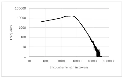
One peculiarity of the data are encounters which are quite long, see Figure 1. The average and the median encounter length was found to be 11676 and 7238 tokens, respectively. In addition, the en-counter length distribution exhibits a long tail. At the upper end there are 1422 encounters (0.63%) with more than 100k tokens and the maximum en-counter length reaches 857k tokens.

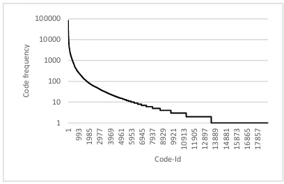
Figure 2 shows the ranked frequency distribu-tion over the target codes. From Figure 2 it is ap-parent that out of the 18846 codes seen in the data about two-thirds appear less than ten times. This code sparsity issue had a direct impact on the sys-tem design as many of the codes can hardly be modeled.

Data preprocessing was kept at a minimum. Af-ter concatenating all EHRs of one encounAf-ter into one document lowercasing was applied. Date and time expressions as well as URLs, phone numbers

and other numerical expressions were

Partition-A Train/Dev

Partition-B Train/Dev

Test

#months of data 6 16 1

#encounters 81k 234k 14.1k

#tokens 0.9G 2.6G 160M

#running codes 870k 2.5M 143k

#codes types 13094 18846 6863

Table 1: Data statistics.

Figure 1: Encounter length distribution. 1

10 100 1000 10000 100000

10 100 1000 10000 100000 1000000

Fr

eq

u

en

cy

canonicalized. Finally, after applying some shallow normalization (hyphens, underscores) tokenization was done using whitespace as token separators.

4

Models and methods

As mentioned in Section 3 we had to operate over a set of codes with a wide range of occurrence probabilities. For some of the target codes training material was abundant whereas for others we were faced by severe data sparsity. To address this issue, we followed a system combination strategy com-bining a set of Logistic Regression (LR) classifiers, with a Convolutional Neural Network (CNN).

To cope with the multi-label nature of the classi-fication problem we applied a first-order modeling strategy tackling the task in a code-by-code manner thus ignoring the coexistence of other codes (Zhang and Zhou, 2014). In case of LR this model-ing strategy was strict, meanmodel-ing that one LR model was built per target code. In the CNN case a relaxed version of this strategy was applied. One common CNN was built, with the target codes modeled con-ditionally independent by the loss function.

Regularized binary cross-entropy was applied for both the LR and the CNN objective function. In all cases model training was followed by a thresh-old tuning step to determine optimal decision thresholds. Finally, all test results are presented in terms of micro-F1 (Wu and Zhou, 2017).

4.1 Logistic regression

LR is a well understood and robust classification method. It is expected to perform well even for low frequency classes. The problem is convex and typ-ically applied in conjunction with a L1 or a L2

regularization, the ‖𝑤‖ term in the LR objective function (1).

min

𝑤 𝐶‖𝑤‖ + ∑ log(1 + 𝑒

−𝑦_𝑖𝑤𝑇𝑥_𝑖) 𝑙

𝑖=1 (1)

For solving the LR problem we used LibLinear (Fan et al., 2008) which is a large-scale linear clas-sification library. The LibLinear solver exhibits the advantage that there is only one free hyperparame-ter to tune, namely the regularization weight 𝐶.

4.2 Convolutional neural networks

Compared to LR a CNN features an increased com-plexity. This higher modeling capability comes though with the need for more training data which makes it more suited for high frequency classes.

The CNN design we applied for this work fol-lows the work described in Kalchbrenner et al. (2014) and Conneau et al. (2016). The basic archi-tecture consists of one convolutional layer which is followed by max-pooling resulting in one feature per convolutional filter and document. As input to the convolutional layer word embeddings apply which were pre-trained using word2vec (Mikolov et al., 2013). The feature extraction layer is suc-ceeded by the classification part of the network consisting of a feed-forward network of one fully-connected hidden layer and the final output layer. The output layer is formed by one node with sig-moid activation for each ICD-10 code, effectively modeling the code’s probability.

Additional convolutional layers are added in conjunction with highway layers connecting each convolutional layer directly with the classification part of the network. The highway connections and the output of the last convolutional layer are fol-lowed by the same max-pooling operation de-scribed above. The convolutional layers are con-nected by a sliding-window max-pooling opera-tion. For each filter of the lower convolutional layer a max-pooling operator of kernel-width 3 is applied to the stream of filter output values. With a stride of one the layer’s output consists of a vector-fea-ture stream which is of the same length as the input token sequence and a vector-dimension equal to the number of filters of the lower convolutional layer. For our CNN implementation Theano (2017) was used. All CNNs were built using a NVIDIA P6000 GPU with 22GByte GPU-memory.

4.3 System combination

System combination was implemented by linearly interpolating the hypothesized predictions from the LR system and the CNN system. The interpolation weights were optimized maximizing dev set micro-F1. In case of codes which were not modeled by the CNN the LR predictions were directly used.

5

Experiments and results

For practical reasons it was not possible to model all CM codes. Most of the 71704 ICD-10-CM codes are never seen in the available data and even many of the seen codes are too rare to be eled, see Figure 2. We therefore restricted our mod-els to the most frequent codes seen within the first seven month of data. For the LR systems we used the most frequent 3000 codes. The CNN was re-stricted to model only the most frequent 1000 codes which reflects the data sparsity issues discussed in Section 3. With these settings a code coverage of >95% for the LR systems and >87 % for the CNN systems was obtained. Table 2 gives detailed code coverage statistics of the training data.

Model testing was directly affected by the target

code restrictions. Out of the 143k running codes of the test set 6189 instances are not covered by the 3000 modeled codes and 71 of the 3000 modeled codes do even not appear in the test set.

The following experiments give results for the most frequent (top) 200, 1000, and 3000 codes and all codes seen in the test set. Note that for the case of 1000 codes and the case of 3000 codes there are 17653 and 6189 code instances, respectively, which are not modeled. These instances always en-tered the F1 calculation as false negatives when scored on all seen codes.

5.1 Basic system development

This phase of the project focused on basic system design question. All experiments were carried out using data-partition A.

In case of the LR system we model a document as a ‘bag-of-ngrams’ up to an ngram-length of three. With a frequency cutoff of 20 this gave 4.1M features. Using higher order ngram-features or a smaller cutoff value didn’t provide any improve-ments. For all LR experiments described in this work indicator features apply.

Table 3 lists the results of two LR systems. Both systems apply the same feature file which is used for all 3000 code specific classifiers. The basic LRa system applies a common regularization weight 𝐶

for all codes. In case of system LRa2 the regulari-zation weight 𝐶 was tuned individually for each code using 4-fold cross-validation over the training set. Tuning the regularization weights resulted in micro-F1 gains of ~0.8% absolute. Using an in-creased fold number didn’t provide any improve-ments.

For the CNN experiments we first used the CNN design with one convolutional layer described in Section 4. After some initial experiments the con-volutional layer of the network was fixed to 900 fil-ters with a filter width of five tokens. The hidden layer was fixed to 1024 nodes and the output layer models the most frequent 1000 ICD-10-CM codes. Max-pooling was followed by Relu-activations.

All models were trained with RMSPROB. The convolutional layer used L2-regularization and L1-regularization was used for the hidden layer and the output layer. Dropout was applied to the output of the max-pool operation. Best results were achieved with a batch size (encounter level) of 32.

The result named CNa1 in Table 3 follows the Top 200/1k/3k and All seen codes

Parti-tion

Data statistics 200 1000 3000 All

A #running codes 560k 768k 836k 870k

A #code coverage 64.4% 88.3% 96.2% 100%

B #running codes 1.6M 2.1M 2.3M 2.5M

B #code coverage 63.3% 87.3% 95.2% 100%

Table 2: Code coverage statistics.

Micro-F1 for the top 200/1k/3k codes and All seen codes

System 200 1000 3000 All

LRa1 70.37 64.03 61.59 60.19

LRa2 71.48 64.81 62.38 60.96

CNa1 73.96 66.31 63.31 61.79

CNa2 74.82 67.25 64.24 62.71

LRa2 & CNa2 75.38 68.61 65.65 64.14

design with one convolutional layer. The CNa1 system was initialized with 50-dimensional word embeddings which were pre-trained on the training data with word2vec (Mikolov et al., 2013). These embeddings were further refined during network training. This gave a final micro-F1 of 66.31% ab-solute when scored over the 1000 modeled codes. Best results were obtained with 50-dimensional embeddings and without batch normalization within the convolutional layer.

In a second step some initial experiments with the two convolutional layers CNN design were car-ried out. This network featured 300 filters and 900 filters in the first and second convolutional layer, respectively. The filter width was set to five and Relu-activations were used for the first layer.

Table 3 shows that the two convolutional layers system CNa2 achieves the best performance of a single system with an absolute increase in micro-F1 of ~0.9% over the CNa1 system with its one convolutional layer. In contrast to the setup with one convolutional layer the use of batch normaliza-tion turned out to be essential in the two-convolu-tional layer setup. Dropping it gave worse results compared to the one-convolutional layer design.

Finally, we explored the combination of the LR approach with the CNN approach. Linearly inter-polating the LRa2 system with the CNa2 system gave the best results with 64.44% micro-F1 (65.37% precision, 63.53% recall) clearly outper-forming the underlying individual systems. We also examined other system combination strategies following the work from Heng et al. (2016). How-ever, the linear interpolation approach described in this work turned out to work best.

Investigating the performance of the LRa2 sys-tem and the CNa2 syssys-tem on code level, we found our assumption confirmed that the CNN is more suited to model high frequency codes whereas the LR system does better for low frequency codes.

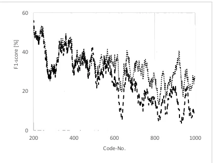
Figure 3 shows that the CNN does better for the most frequent 200 codes. However, after a transi-tion region covering roughly the next 300 codes, the LR system starts to outperform the CNN

sys-tem consistently, starting approximately from code position 500 on, see Figure 4.

These finding were reconfirmed when checking for the relative improvements of the combined LRa2 & CNa2 system over the CNa2 system. Comparing the scores for the most frequent 200 codes and the most frequent 1000 codes one finds 0.75% and 2.02% relative improvements, respec-tively. The LR system also fills up the 2000 codes not modeled by the CNN giving in a relative micro-F1 win of 2.19% when scoring over 3000 codes.

An integral part of the model building process was the tuning of the decision thresholds. Though individual thresholds per code are possible best mi-cro-F1 results were always achieved with a com-mon decision threshold over all codes. This behav-ior reflects again the data sparsity issues as not all modeled codes appear in the dev set and many other codes are so sparse that no robust threshold estimation was possible.

5.2 System refinements

In this phase of the project we focused on improved training recipes and the use of more training data given by data-partition B. We kept on modeling the same set of codes as used in Section 5.2. This lead Figure 3: F1-scores, top 200 codes, CNN

(dashed line) versus LR (dotted line). 45

55 65 75 85 95

0 40 80 120 160 200

F1

-s

co

re

[%

]

Code-No.

Figure 4: F1-scores, top 201-1000 codes, CNN (dashed line) versus LR (dotted line) 0

20 40 60

200 400 600 800 1000

F1

-s

co

re

[%

]

Code-No.

to a slight reduction in code coverage, see Table 2, but guaranteed the comparability of the results.

For LR a bootstrapping approach was followed aiming to refine the system step-by-step from one model to the next model. We built up on the train-ing recipe used to build system LRa2, see Section 5.1, i.e. L1 regularized LR with per-code tuned reg-ularization constants 𝐶. First, we switched to the larger data-partition B which added additional 10 months of data to the original 6 months of data. Comparing the resulting LRb1 system with the LRa2 system, see Table 4, we found that the addi-tional data improved micro-F1 by ~1.2% absolute. The use of more data increased the features space from 4.1M features to 9.2M features. To ease subsequent development work, we applied a fea-ture reduction approach taking advantage of the feature selection property of the L1 regularization (Andrew Ng, 2004). Reducing the feature space of the LRb1 system to all features with none-zero model weights reduced the features space by a fac-tor of 62 giving 149k features. This feature selec-tion step also improved system performance by ~0.2% absolute micro-F1, see LRb2 in Table 4.

LR is a linear classification method fitting a hy-perplane as decision boundary into feature space. To leverage the increased modeling capabilities of a none-linear modeling regime, we applied a quad-ratic kernel to the feature space. With a features di-mension of 149k this is yet a prohibitive endeavor. Instead we used code specific reduced features spaces. Based on the most prominent 400 features per code the quadratic kernel was applied which gave up to 80.2k squared features per code. After model building these features spaces were reduced again to all features with none-zero model weights.

2 _{At the time of writing this paper the results for the} 2-con-volutional layer CNN which was built on the partition B

Table 4 lists the corresponding results as LRb3. For the most frequent 200 codes absolute micro-F1 im-provements of ~0.7% are observed with respect to the LRb2 system. For the less frequent codes this effect is nearly washed out though.

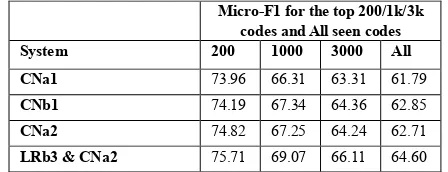
The partition B data was also applied to the CNN. Table 5 compares the corresponding 1-con-volutional layer system built on the partition B data with the CNNs built on the partition A data2_{. We}

found that the additional 10 month of training data provide a ~0.2% - ~1% improvement in absolute micro-F1. Note that system CNb1 outperforms sys-tem CNa2 when soring over all 1000 modeled codes but that system CNa2 is better when scoring only over the top 200 codes, see Table 5. We attrib-ute this behavior to the change in the code distribu-tion when switching from partidistribu-tion A to partidistribu-tion B.

Finally, the best LR system, LRb3, was com-bined with the CNa2 system giving the best overall results with a micro-F1 of 64.60% (68.10% preci-sion, 61.60% recall). Compared to the best single systems, CNa2 and CNb1, absolute micro-F1 im-provements of ~1.8% - ~1.9% are observed.

6

Conclusions

In this work we have presented our work on build-ing a machine learnable CAC system. The focus lies on aspects developers are faced with in prac-tice. Data peculiarities like data amount, imbal-ances in code frequencies or sample length were discussed. We provide evidence that the imbal-ance issues are best addressed by a dedicated modeling approach for each datatype. Finally, with our combined LR-CNN system which mod-els 3000 ICD-10-CM codes we achieved a micro-Micro-F1 for the top 200/1k/3k

codes and All seen codes

System #features 200 1000 3000 All

LRa2 4.1M 71.48 64.81 62.38 60.96

LRb1 9.2M 72.62 66.18 63.83 62.39

LRb2 149k 72.78 66.41 64.05 62.59

LRb3 7 - 5113 73.45 66.70 64.18 62.72

Table 4: Partition-B LR test results. LRa2: Partition-A reference system; LRb1: Same as LRa2 but with Phase-B data; LRb2: Same as LRb1 but with feature reduction; LRb3: sys-tem with per-code quadratic-kernel features.

Micro-F1 for the top 200/1k/3k codes and All seen codes

System 200 1000 3000 All

CNa1 73.96 66.31 63.31 61.79

CNb1 74.19 67.34 64.36 62.85

CNa2 74.82 67.25 64.24 62.71

LRb3 & CNa2 75.71 69.07 66.11 64.60

F1 score of 64.60% when scored over all codes seen in the test set.

References

Alexis Conneau, Holger Schwenk, Loïc Barrault, Yann Lecun, Very Deep Convolutional Networks for Text Classification. In Proceedings of the 15th

Confer-ence of the European Chapter of the Association for Computational Linguistics, 2016, pages 1107-1116.

https://arxiv.org/pdf/1606.01781.pdf

Andrew Ng, Feature selection, L1 vs. L2 regulariza-tion, and rotational invariance. In Proceedings of the 21st International Conference on Machine Learn-ing, Association for Computational Linguistics, 2004, page 78. http://ai.stanford.edu/~ang/pa-pers/icml04-l1l2.pdf

A. Perotte, R. Pivovarov, K. Natarajan, N. Weiskopf, F. Wood, N. Elhadad, 2014, Diagnosis code assign-ment: models and evaluation metrics. In the Journal of the American Medical Informatics Association.

https://www.ncbi.nlm.nih.gov/pmc/arti-cles/PMC3932472/pdf/amiajnl-2013-002159.pdf

Diagnosis-related group. Design and development of the Diagnosis Related Group (DRG).

https://www.cms.gov/

Elyne Scheurwegs, Boris Cule, Kim Luyckx, Léon Luyten, Walter Daelemans, Selecting Relevant Fea-tures from the Electronic Health Record for Clinical Code Prediction. Preprint submitted to Journal of

Biomedical Informatics, 2017.

http://win.ua.ac.be/~adrem/bibrem/pubs/confcov.pdf

Elyne Scheurwegs, Kim Luyckx, Léon Luyten, Walter Daelemans, Tim Van den Bulcke, Data integration of structured and unstructured sources for assigning clinical codes to patient stays. In the Journal of the American Medical Informatics Association, 2015

https://www.clips.uantwerpen.be/~walter/pa-pers/2015/slldv15.pdf

Haoran Shi, Pengtao Xie, Zhiting Hu, Ming Zhang, Eric Xing, Towards Automated ICD Coding Using Deep Learning. In https://arxiv.org/, 2018.

https://arxiv.org/pdf/1711.04075.pdf

Heng-Tze Cheng, Levent Koc, Jeremiah Harmsen, Tal Shaked, Tushar Chandra, Hrishi Aradhye, Glen An-derson, Greg Corrado, Wei Chai, Mustafa Ispir, Ro-han Anil, Zakaria Haque, LicRo-han Hong, ViRo-han Jain, Xiaobing Liu, Hemal Shah. Wide & Deep Learning for Recommender Systems. In https://arxiv.org/, 2016, https://arxiv.org/pdf/1606.07792.pdf I. Goldstein, A. Arzumtsyan, O. Uzuner, Three

Ap-proaches to Automatic Assignment of ICD-9-CM Codes to Radiology Reports, In AMIA Annual Sym-posium Proceedings, 2007, pages 279–283,

https://www.ncbi.nlm.nih.gov/pmc/arti-cles/PMC2655861/pdf/amia-0279-s2007.pdf

M. L. Zhang, Z. H. Zhou, A review on multi-label learning algorithms, In IEEE Transactions on

Knowledge and Data Engineering, 2014, pages 1819-1837.

http://ieeex-plore.ieee.org/stamp/stamp.jsp?arnumber=6471714

Nal Kalchbrenner, Edward Grefenstette, Phil Blunsom, Phil, A Convolutional Neural Network for Modeling Sentences. In Proceedings of the 52nd _Annual

Meet-ing of the Association for Computational LMeet-inguistics (Volume 1: Long Papers), Association for Compu-tational Linguistics, 2014, pages 655-665.

https://arxiv.org/pdf/1404.2188.pdf

N. G. Weiskopf, G. Hripcsak, S. Swaminathan,C. Weng, Defining and measuring completeness of electronic health records for secondary use. In Jour-nal of Biomedical Informatics, 2013.

https://www.ncbi.nlm.nih.gov/pmc/arti-cles/PMC3810243/

R. Cohen, M. Elhadad, N. Elhadad, Redundancy in electronic health record corpora: analysis, impact on text mining performance and mitigation strategies, In BMC Bioinformatics, 2013. https://bmcbioinfor-

matics.biomedcentral.com/articles/10.1186/1471-2105-14-10

Richárd Farkas, György Szarvas, Automatic construc-tion of rule-based ICD-9-CM coding systems, In

BMC Bioinformatics, 2008, https://bmcbioinfor- matics.biomedcentral.com/articles/10.1186/1471-2105-9-S3-S10

R.-E. Fan, K.-W. Chang, C.-J. Hsieh, X.-R. Wang, and C.-J. Lin, LIBLINEAR: A library for large linear classification. In Journal of Machine Learning

Re-search, 2008, pages 1871-1874.

https://www.csie.ntu.edu.tw/~cjlin/papers/liblin-ear.pdf

R. Miotto, L. Li, B. A. Kidd, J. T. Dudley, Deep Patient: An Unsupervised Representation to Predict the Fu-ture of Patients from the Electronic Health Records. In Nature Scientific Reports, 2016

https://www.na-ture.com/articles/srep26094/

S. Pakhomov, J. D. Buntrock, C. G. Chute, Automating the Assignment of Diagnosis Codes to Patient Encounters Using Example-based and Machine Learning Techniques. In the Journal of the American Medical Informatics Association, 2006.

https://www.ncbi.nlm.nih.gov/pmc/arti-cles/PMC1561792/pdf/516.06001186.pdf

Theano, http://deeplearning.net/software/theano/ Tomas Mikolov, Kai Chen, Greg Corrado, Jeffrey

Dean, Efficient Estimation of Word Representations in Vector Space. In, ICLR Workshop, 2013.

https://arxiv.org/pdf/1301.3781.pdf

World Health Organization ICD. World Health Organ-ization, International classification of diseases,

http://www.who.int/classifications/icd/en/

Xi-Zhu Wu 1 Zhi-Hua Zhou, A Unified View of Multi-Label Performance Measures, In https://arxiv.org/, 2017. https://arxiv.org/pdf/1609.00288.pdf