Abstract—In this paper a singly diagonally implicit Runge-Kutta-Nyström (RKN) method is developed for second-order ordinary differential equations with periodical solutions. The method has algebraic order four and phase-lag order eight at a cost of four function evaluations per step. This new method is more accurate when compared with current methods of similar type for the numerical integration of second-order differential equations with periodic solutions, using constant step size.
Keywords—Runge-Kutta-Nyström methods; Diagonally implicit; Phase-lag; Oscillatory solutions.
I. INTRODUCTION
HIS paper deals with numerical method for second-order ODEs, in which the derivative does not appear explicitly,
0 0 0 0
( ) ( ) ( )
y f x y y x y y x y (1) for which it is known in advance that their solution is oscillating. Such problems often arise in different areas of engineering and applied sciences such as celestial mechanics, quantum mechanics, elastodynamics, theoretical physics and chemistry, and electronics. An s-stage Runge-Kutta-Nyström (RKN) method for the numerical integration of the IVP is given by
2 1
1
1
1
s
n n n i i
i s
i i
n n
i
y
y
h
y
h
b k
h
b k
y
y
(2)Manuscript received May, 2011; revised May , 2011. This work was supported in part by the UPM Research University Grant Scheme (RUGS) under Grant 05-01-10-0900RU and Fundamental Research Grant Scheme (FRGS) under Grant 01-07-10-917FR
N. Senu is with the Department of Mathematics and Institute for Mathematical Research, Universiti Putra Malaysia, 43400 UPM Serdang, Selangor, MALAYSIA. (corresponding author phone: 603-8946-6848; fax: 603-89437958; e-mail: [email protected] ).
M. Suleiman and F. Ismail are with Department of Mathematics and Institute for Mathematical Research, Universiti Putra Malaysia,
43400 UPM Serdang, Selangor, MALAYSIA. (e-mail: [email protected], [email protected] ).
M. Othman is with the Institute for Mathematical Research, Universiti Putra Malaysia, 43400 UPM Serdang, Selangor, MALAYSIA.
(e-mail: [email protected]).
where
2 1
1 s
i n i n i n ij j
j
k f x c h y c hy h a k i s
The RKN parameters a b bij j j andcj are assumed to be real and s is the number of stages of the method. Introduce the s -dimensional vectors c b and b ands s matrix A, where
1 2
[ ]T
s
c c c c [ 1 2 ]T s
b b b b [ 1 2 ]T s
b b b b
[ ij]
A a respectively. RKN methods can be divided into two broad classes: explicit (ajk 0, k j ) and implicit (ajk 0, k > j). The latter contains the class of diagonally implicit RKN (DIRKN) methods for which all the entries in the diagonal of A are equal. The RKN method above can be expressed in Butcher notation by the table of coefficients
c A T
b T
b
Generally problems of the form (1) which have periodic solutions can be divided into two classes. The first class consists of problems for which the solution period is known a priori. The second class consists of problems for which the solution period is initially unknown. Several numerical methods of various types have been proposed for the integration of both classes of problems. See Stiefel and Bettis [3], van der Houwen and Sommeijer [12], Gautschi [16] and others.
When solving (1) numerically, attention has to be given to the algebraic order of the method used, since this is the main criterion for achieving high accuracy. Therefore, it is desirable to have a lower stage RKN method with maximal order. This will lessen the computational cost. If it is initially known that the solution of (1) is of periodic nature then it is essential to consider phase-lag (or dispersion) and amplification (or dissipation). These are actually two types of truncation errors. The first is the angle between the true and the approximated solution, while the second is the distance from a standard cyclic solution. In this paper we will derive a new diagonally implicit RKN method with four-stage fourth-order with dispersion of order eight.
A Singly Diagonally Implicit
Runge-Kutta-Nyström Method for Solving Oscillatory
Problems
N. Senu, M. Suleiman, F. Ismail, and M. Othman
T
IAENG International Journal of Applied Mathematics, 41:2, IJAM_41_2_11
A number of numerical methods for this class of problems of the explicit and implicit type have been extensively developed. For example, Okunbor and Skeel [1], van der Houwen and Sommeijer [12], Simos, Dimas and Sideridis, [15], and Senu, Suleiman and Ismail [18] have developed explicit RKN methods of algebraic order up to six for solving oscillatory problems. For implicit RKN methods, see for example van der Houwen and Sommeijer [13], Sharp, Fine and Burrage [14], Imoni, Otunta and Ramamohan [17] and Senu, Suleiman, Ismail, and Othman [21] and [23], and Al-Khasawneh, Ismail, Suleiman [22] and [24].
In this paper a dispersion relation is imposed and together with algebraic conditions to be solved explicitly. In the following section the construction of the new four-stage fourth-order diagonally implicit RKN method with dispersion of order eight is described. Its coefficients are given using the Butcher tableau notation. Finally, numerical tests on second order differential equation problems possessing an oscillatory solutions are performed.
II. ANALYSIS OF PHASE-LAG AND STABILITY
In this section we shall discuss the analysis of phase-lag for RKN method. The first analysis of phase-lag was carried out by Bursa and Nigro [10]. Then followed by Gladwell and Thomas [5] for the linear multistep method, and for explicit and implicit Runge-Kutta(-Nystrom) methods by van der Houwen and Sommeijer [12], [13]. The phase analysis can be divided in two parts; inhomogeneous and homogeneous components. Following van der Houwen and Sommeijer [12], inhomogeneous phase error is constant in time, meanwhile the homogeneous phase errors are accumulated as n increases. Thus, from that point of view we will confine our analysis to the phase-lag of homogeneous component only.
The phase-lag analysis of the method (2) is investigated using the homogeneous test equation
2 ( ) ( )
y i y t (3) Alternatively the method (2) can be written as
2 1 1 1 1 ( ) ( ) s
n n n i n i i
i s
i n i i
n n
i
y y hy h b f t c h Y
h f t c h Y
y y b
(4)where
2 1
( )
s
i n i i ij n i j
j
Y y c hy h a f t c h Y
By applying the general method (2) to the test equation (3) we obtain the following recursive relation as shown by Papageorgiou, Famelis and Tsitouras [4]
1 1
n n
n n
y y
D z h
hy hy
, 1 1 1 1
1 ( ) 1 ( )
( )
( ) 1 ( )
T T
T T
Hb I HA e Hb I HA c
D H
Hb I HA e Hb I HA c
(5)
where 2
1 (1 1)T ( )T
m
H z e c cc . Here D(H) is the stability matix of the RKN method and its characteristic polynomial
2 2 2
tr( (D z )) det( (D z )) 0,
(6)
is the stability polynomial of the RKN method. Solving difference system (5), the computed solution is given by
2 ncos( )
n
y c n (7) The exact solution of (3) is given by
( )n 2 cos( )
y t nz (8) Eq. (7) and (8) led us to the following definition.
Definition 1. (Phase-lag). Apply the RKN method (2) to (3). Then we define the phase-lag ( )z z . If ( )z O z( q1), then the RKN method is said to have phase-lag order q . Additionally, the quantity ( )z 1 is called amplification error. If ( )z O z( r1), then the RKN method is said to have dissipation order r .
Let us denote
2 2
( ) trace( ) and ( ) det( )
R z D S z D
From Definition 1, it follows that 2
1 2
2 ( )
( ) cos ( )
2 ( )
R z
z z S z
S z
Let us denote R z( 2) and S z( 2) in the following form
2 2 2 1 2 2 ( ) ˆ (1 + )
s s s z z R z z
(9)
2 2 2 1 2 1 ( ) , ˆ (1 + )
s s s z z S z z
(10)
where ˆ22 is diagonal element in the Butcher tableau. Here the necessary condition for the fourth-order accurate diagonally implicit RKN method (2) to have phase-lag order eight in terms of i and i is given by
2 6 4 3 3 2 1 32 24 3 360
(11)
IAENG International Journal of Applied Mathematics, 41:2, IJAM_41_2_11
2
8 4
3 4 4
1 14 3
16 10
2 45 2240
(12)
Notice that the fourth-order method is already dispersive order four and dissipative order five due to consistency of the method. Furthermore dispersive order is even and dissipative order is odd.
We next discuss the stability properties of method for solving (1) by considering the scalar test problem (3) applied to the method (4), from which the expression given in (5) is obtain. Eliminating yn and yn1 in (5), we obtain a difference
equation of the form
2 ( ) 1 ( ) 0
n n n
y R H y S H y (13)
The characteristic equation associated with equation (13) is given as in (6). Chawla and Sharma [11] have discussed the interval of periodicity and absolute stability of Nyström method. Since our concerned here is with the analysis of high order dispersive RKN method, we therefore drop the necessary condition of periodicity interval i.e (S H)1. Hence the method derived will be with empty interval of periodicity. We now consider the interval of absolute stability of RKN method. We therefore need the characteristic equation (6) to have roots with modulus less than one so that approximate solution will converge to zero as n tends to infinity. For convenience, we note the following definition adopted for method (5).
Definition 2. An interval (Ha0) is called the interval of absolute stability of the method (5) if, for all H ( Ha0),
1 2 1
.
III. CONSTRUCTION OF THE METHOD
In the following we shall derive a four-stage fourth-order accurate diagonally implicit RKN method with dispersive order eight, by taking into account the dispersion relations in section II. The RKN parameters must satisfy the following algebraic conditions to find fourth-order accuracy as given in Hairer and Wanner [2], Butcher [6] and Dormand [9].
order 1
1 i
b
(14) order 21 1
2 2
i i i
b b c
(15) order 32
1 1 1
6 2 6
i i i i
b c b c
(16)order 4
2 3
1 1 1 1 1
2
b ci i 24 6
b ci i 24
b a ci ij j 24. (17)For most methods the
c
i need to satisfy2 1 1
( 1 )
2 s
i ij
j
c a i s
(18)
A four-stage method of algebraic order four (p4) with dispersive order eight (q8) and dissipative order five (r5) is now considered. The conditions (14)-(18) and dispersion relations (11)-(12) formed thirteen nonlinear equations with nineteen variables to be solved. Now, from algebraic conditions (14)-(18) and phase-lag relations of order six (11) and letting be a free parameter, then we solve it simultaneously. Therefore the following solution of one-parameter family is obtained
2
1 2 3 4 21
2 2
32 43 31 41 42
2
11 22 33 44 1 1 2 3
2
2 2 3 2
2
4
1 3 1 3 1 3 1 3
2 2
2 6 2 6 2 6 6 12
1 3 1 3
2 2 0
6 12 6 12
1 3
2 0
4 12 3(80 1)
10( 3 3 24 3 24 12 3 288 72 )
1 60 3 15
c c c c a
a a a a a
a a a a b b b b b
b
2 5 3 360 3 120 33 3 2
5( 3 3 24 3 24 12 3 288 72 )
From the above solution, we are going to derive a method with dispersion of order eight. The eight order dispersion relation (12) need to be satisfied and this can be written in terms of RKN parameters which corresponds to the above family of solution yields the following equation
7 6 6 5 5
4 4 3 3 2 2
(5806080 1451520 1451520 3 241920 3 967680
60480 181440 3 80640 3 147168 44856 29736 3
924 3 1752 585 349 3) [120960(12 3 3)] 0 0
and solving for yields
-0.2752157925, -0.08524516029, 0.04719733276, 0.1682412065, 0.2490198846, 0.6846776634, and
-0.1056624327.
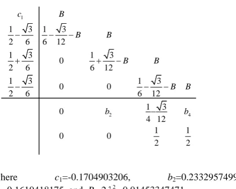
Numerical results show that choosing -0.08524516029 will give us more accurate scheme compared to the others and we mentioned here one fourth-order (p=4) with dispersive order eight (q=8) method. For -0.08524516029, the following method will be produced. This method will be denoted by DIRKN4(4,8)NEW (see Table I) and its stability interval is approximately (-8.1877,0).
IAENG International Journal of Applied Mathematics, 41:2, IJAM_41_2_11
Table 1: : The DIRKN3(4,6) method
where c1=-0.1704903206, b2=0.2332957499, b4=0.1610418175, and B=22=0.01453347471.
This method has PLTE
(5)
(5) 3 3
2
1 669237 10 and 1 611272 10
.
Table II compares the properties of our method with the methods derived by van der Houwen and Sommeijer [20], Sharp, Fine and Burrage [14], Imoni, Otunta and Ramamohan [17] and Al-Khasawneh, Ismail and Suleiman [22].
IV. PROBLEM TESTED
In this section we use our method to solve homogeneous and inhomogeneous problems whose exact solution consists of a rapidly or/and a slowly oscillating function. For purposes of illustration, we will compare our results with those derived by using four methods; DIRKN three-stage fourth-order derived by van der Houwen and Sommeijer [20] and Imoni, Otunta, Ramamohan [17], three-stage fourth-order dispersive order six derived by Sharp, Fine and Burrage [14] and four-stage fourth-order derived by Al-Khasawneh, Ismail, Suleiman [22].
Problem 1(Homogenous) 2
2 ( )
100 ( ) (0) 1 (0) 2
d y t
y t y y
dt
Exact solution 1 5
( ) sin(10 ) cos(10 )
y t t t
Problem 2 (Inhomogenous) 2
2 ( )
( ) (0) 1 (0) 2
d y t
y t t y y
dt
Exact solution ( )y t sin( ) cos( )t t t Source : Allen and Wing [19]
Problem 3(Inhomogeneous system) 2 2 2 1 1 2 1 1 2 2 2 2 2 2 2 2 ( ) ( ) ( ) ( )
(0) (0) (0) (0)
( )
( ) ( ) ( )
(0) (0) (0) (0)
d y t
v y x v f t f t
dt
y a f y f
d y t
v y t v f t f t dt
y f y va f
Exact solution is
1( ) cos( ) ( ) 2( ) sin( ) ( )
y t a vt f t y t a vt f t ( )f t is chosen to be e 0 05t and parameters v and a are 20 and 0.1 respectively.
Source : Lambert and Watson [7]
Problem 4 (An almost Periodic Orbit problem)
2 1
1 1 1
2 2
2
2 2 2
2 ( )
( ) 0 001cos( ) (0) 1 (0) 0 ( )
( ) 0 001sin( ) (0) 0 (0) 0 9995
d y t
y t t y y
dt d y t
y t t y y
dt
Exact solution y t1( )cos( )t 0 0005 sin( )t t , 2( ) sin( ) 0 0005 cos( )
y t t t t
Source : Stiefel and Bettis [3]
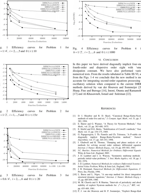
The following notations are used in Tables III-VI and Figs. 1-4:
DIRKN4(4,8)NEW : A four-stage fourth-order dispersive order eight method with ’small’ dissipation constant derived in this paper.
DIRKN3(4,4)IMONI : A three-stage fourth-order derived by Imoni, Otunta and Ramamohan [17]. DIRKN3(4,4)HS : A three-stage fourth-order
dispersive order four derived by van der Houwen and Sommeijer [20].
DIRKN3(4,6)SHARP : A three-stage fourth-order dispersive order six as in Sharp, Fine and Burrage [14].
TABLEI THE DIRKN4(4,8)NEW METHOD
1
2 4
1 3 1 3
2 6 6 12
1 3 1 3
0
2 6 6 12
1 3 1 3
0 0
2 6 6 12
1 3 0 4 12 1 1 0 0 2 2 c B B B B B B B b b TABLEII
SUMMARY OF THE CHARACTERISTIC OF THE FOURTH-ORDER DIRKN
METHODS
Method q d ( 1)
2
p
( 1)
2
p
DIRKN4(4,8)NEW 8 5
4.84 10 3
1 67 10 3
1 61 10
DIRKN3(4,4)IMONI 4 - 2
3 75 10 2
3 22 10
DIRKN3(4,4)HS 4 4
1 43 10 4
6 35 10 4
1 59 10
DIRKN3(4,6)SHARP 6 2
1 02 10 3
1 85 10 4
6 26 10
DIRKN4(4,4)RAED 4 2
1 80 10
2
3.13 10 2
1 71 10 Notations : q – Dispersion order, d – Dissipation constant
( 1) 2
p
– Error coefficient for yn
( 1) 2
p
– Error coefficient for yn
IAENG International Journal of Applied Mathematics, 41:2, IJAM_41_2_11
DIRKN4(4,4)RAED : A four-stage fourth-order drived by Al-Khasawneh, Ismail, Suleiman [22].
V. NUMERICAL RESULTS
The results for the four problems above are tabulated in Tables III-VI. One measure of the accuracy of a method is to examine the Emax(T), the maximum error which is defined by
Emax( )T maxy t( )n yn
0 0
wheretn t nh n 1 2? T t h
Tables III-VI show the absolute maximum error for DIRKN4(4,8)NEW, DIRKN3(4,4)IMONI, DIRKN3(4,4)HS, DIRKN3(4,6)SHARP and DIRKN4(4,4)RAED methods when solving Problems 1-4 with three different step values. From numerical results in Table III-VI, we observed that the new method is more accurate compared with DIRKN3(4,4)IMONI, DIRKN3(4,4)HS and DIRKN4(4,4)RAED methods which do not relate to the dispersion order of the method. Also the new method is more accurate compared with DIRKN3(4,6)SHARP method because the new method has dispersion order eight which is the highest and also the dissipation constant for our method is small (see Table II). Notice that all the methods are of the same algebraic order.
Figs. 1-4 show the decimal logarithm of the maximum global error for the solution (MAXE) versus the number of function evaluations. From Figs. 1-4, it can be seen that for the same number of function evaluations the new DIRKN4(4,8)NEW method is more accurate when compared to the current same type and the same order of DIRKN methods, DIRKN4(4,4)RAED, DIRKN3(4,4)HS, DIRKN3(4,6)SHARP and DIRKN3(4,4)IMONI.
TABLE III
COMPARING OUR RESULTS WITH THE METHODS IN THE LITERATURE FOR
PROBLEM 1
h Method T=100 T=1000 T=4000
0.0025 DIRKN4(4,8)NEW 1.4194(-9) 1.0464(-7) 7.7266(-7)
DIRKN3(4,4)IMONI 1.5646(-2) 1.4622(-1) 4.7069(-1)
DIRKN3(4,4)HS 1.2561(-7) 1.3689(-6) 5.8314(-6)
DIRKN3(4,6)SHARP 3.0150(-7) 3.0229(-6) 1.2120(-5)
DIRKN4(4,4)RAED 9.2774(-6) 9.2904(-5) 3.7129(-4)
0.005 DIRKN4(4,8)NEW 1.5124(-9) 1.5126(-8) 5.3047(-7)
DIRKN3(4,4)IMONI 2.0121(-2) 1.8480(-1) 5.6322(-1)
DIRKN3(4,4)HS 6.6977(-7) 6.6966(-6) 2.7338(-5)
DIRKN3(4,6)SHARP 2.5569(-6) 2.5624(-5) 1.0255(-4)
DIRKN4(4,4)RAED 1.4811(-4) 1.4849(-3) 5.9392(-3)
0.01 DIRKN4(4,8)NEW 4.5984(-8) 4.1025(-7) 1.875664(-6)
DIRKN3(4,4)IMONI 5.9680(-2) 4.6223(-1) 9.286052(-1)
DIRKN3(4,4)HS 3.2305(-5) 3.2361(-4) 1.295597(-3)
DIRKN3(4,6) SHARP 3.1342(-4) 3.1448(-3) 1.263707(-2)
DIRKN4(4,4)RAED 2.3699(-3) 2.3786(-2) 9.536865(-2)
TABLEIV
COMPARING OUR RESULTS WITH THE METHODS IN THE LITERATURE FOR
PROBLEM 2
h Method T=100 T=1000 T=4000
0.065 DIRKN4(4,8)NEW 2.4682(-8) 2.7634(-8) 3.8789(-8)
DIRKN3(4,4)IMONI 5.2936(-3) 5.3213(-2) 2.0104(-1)
DIRKN3(4,4)HS 6.8021(-7) 6.8361(-6) 2.7394(-5)
DIRKN3(4,6) SHARP 4.0017(-6) 4.1061(-5) 1.6419(-4)
DIRKN4(4,4)RAED 5.8594(-5) 5.8706(-4) 2.3509(-3)
0.125 DIRKN4(4,8)NEW 3.4752(-7) 5.1872(-7) 1.0986(-6)
DIRKN3(4,4)IMONI 1.0214(-2) 1.01103(-1) 3.6319(-1)
DIRKN3(4,4)HS 1.0871(-5) 1.0930(-4) 4.3835(-4)
DIRKN3(4,6)SHARP 1.3006(-4) 1.3398(-3) 5.3657(-3) DIRKN4(4,4)RAED 8.0270(-4) 8.0329(-3) 3.2192(-2)
0.25 DIRKN4(4,8)NEW 5.8948(-6) 1.2772(-5) 3.5775(-5)
DIRKN3(4,4)IMONI 1.9124(-2) 1.8683(-1) 6.2958(-1)
DIRKN3(4,4)HS 1.7332(-4) 1.7444(-3) 7.0007(-3)
DIRKN3(4,6) SHARP 4.4802(-3) 4.6441(-2) 1.9520(-1) DIRKN4(4,4)RAED 1.2897(-2) 1.2969(-1) 5.3226(-1)
TABLE V
COMPARING OUR RESULTS WITH THE METHODS IN THE LITERATURE FOR
PROBLEM 3
h Method T=100 T=1000 T=4000 0.0025 DIRKN4(4,8)NEW 8.6798(-10) 2.0910(-8) 1.5309(-7)
DIRKN3(4,4)IMONI 5.9756(-3) 4.6003(-2) 9.1502(-2)
DIRKN3(4,4)HS 3.9675(-7) 3.9897(-6) 1.6028(-5)
DIRKN3(4,6)SHARP 1.8995(-6) 1.9004(-5) 7.6048(-5)
DIRKN4(4,4)RAED 2.9121(-5) 2.9123(-4) 1.1650(-3)
0.005 DIRKN4(4,8)NEW 2.1642(-8) 9.4393(-8) 4.1014(-7)
DIRKN3(4,4)IMONI 1.1371(-2) 7.0105(-2) 9.9201(-2)
DIRKN3(4,4)HS 6.3468(-6) 6.3496(-5) 2.5414(-4)
DIRKN3(4,6)SHARP 6.1529(-5) 6.1776(-4) 2.4938(-3)
DIRKN4(4,4)RAED 4.6623(-4) 4.6689(-3) 1.8754(-2)
0.01 DIRKN4(4,8)NEW 5.1541(-7) 3.4561(-6) 1.3384(-5)
DIRKN3(4,4)IMONI 1.9988(-2) 9.0402(-2) 1.0002(-1)
DIRKN3(4,4)HS 1.0142(-4) 1.0156(-3) 4.0589(-3)
DIRKN3(4,6) SHARP 2.0819(-3) 2.2852(-2) 1.2662(-1) DIRKN4(4,4)RAED 7.5063(-3) 7.7409(-2) 2.5731(-1)
TABLE VI
COMPARING OUR RESULTS WITH THE METHODS IN THE LITERATURE FOR
PROBLEM 4
h Method T=100 T=1000 T=4000
0.065 DIRKN4(4,8)NEW 2.4953(-8) 2.7438(-8) 4.6060(-8)
DIRKN3(4,4)IMONI 3.9398(-3) 4.0219(-2) 2.1108(-1)
DIRKN3(4,4)HS 5.6025(-7) 5.8308(-6) 3.2036(-5)
DIRKN3(4,6) SHARP 3.4938(-6) 3.6382(-5) 1.9990(-4)
DIRKN4(4,4)RAED 4.1138(-5) 4.2777(-4) 2.3486(-3)
0.125 DIRKN4(4,8)NEW 3.5178(-7) 4.8299(-7) 1.2310(-6) DIRKN3(4,4)IMONI 7.3190(-3) 7.3627(-2) 3.7216(-1)
DIRKN3(4,4)HS 7.6595(-6) 7.9664(-5) 4.3794(-4)
DIRKN3(4,6)SHARP 9.3794(-5) 9.7492(-4) 5.3673(-3)
DIRKN4(4,4)RAED 5.6329(-4) 5.8856(-3) 3.2103(-2)
0.25 DIRKN4(4,8)NEW 5.8234(-6) 1.0223(-5) 3.6041(-5)
DIRKN3(4,4)IMONI 1.3995(-2) 1.3655(-1) 6.7067(-1)
DIRKN3(4,4)HS 1.2220(-4) 1.2725(-3) 7.0099(-3)
DIRKN3(4,6) SHARP 3.2209(-3) 3.3895(-2) 1.9396(-1)
DIRKN4(4,4)RAED 9.0479(-3) 9.4159(-2) 5.1301(-1)
Notation : 1.2345(-4) means 1 2345 10 4
IAENG International Journal of Applied Mathematics, 41:2, IJAM_41_2_11
Fig. 1 Efficiency curves for Problem 1 for 1/ 4 ,i 2,..., 5
h i and 0 t 10
Fig. 2 Efficiency curves for Problem 2 for 1/ 2 ,i 1,..., 5
h i and 0 t 15
Fig. 3 Efficiency curves for Problem 3 for 0.6 / 4 ,i 2,..., 6
h i and 0 t 20
Fig. 4 Efficiency curves for Problem 4 for 1/ 2 ,i 2,..., 6
h i and 0 t 1000
VI. CONCLUSION
In this paper we have derived diagonally implicit four-stage fourth-order and dispersive order eight with ‘small’ dissipation constant. We have also performed various numerical tests. From the results tabulated in Table III-VI, and from the Figs. 1-4 we conclude that the new method is more accurate for integrating second-order equations possessing an oscillatory solution when compared to the current DIRKN methods derived by van der Houwen and Sommeijer [20], Sharp, Fine and Burrage [14], Imoni, Otunta and Ramamohan [17] and Al-Khasawneh, Ismail and Suleiman [22].
REFERENCES
[1] D. I. Okunbor and R. D. Skeel, “Canonical Runge-Kutta-Nyström methods of order five and six,” J. Comput. Appl. Math., vol. 51, pp. 375-382, 1994.
[2] E. Hairer and G. Wanner, “A Theory for Nystrom Methods,” Numer.
Math., vol.25, pp. 383-400, 1975.
[3] E. Stiefel and D.G. Bettis, “Stabilization of Cowell’s methods,” Numer.
Math, vol. 13, pp. 154-175, 1969.
[4] G. Papageorgiou, I. Th. Famelis and Ch. Tsitouras, “A P-stable single diagonally implicit Runge-Kutta-Nyström method,” Numerical
Algorithms, vol. 17, pp. 345-353, 1998.
[5] I. Gladwell and R. Thomas, “Damping and phase analysis of some methods for solving second order ordinary differential equations,”
Internat. J. Numer. Methods Engrg., vol. 19, pp. 495-503, 1983.
[6] J.C. Butcher, Numerical Methods for Ordinary Differential Equations, Wiley & Sons Ltd., England, 2003.
[7] J. D. Lambert and I. A. Watson, “Symmetric multistep methods for periodic initial-value problems,” J. Inst. Maths Applics, vol. 18, pp. 189-202, 1976.
[8] J. D. Lambert, Numerical Methods for ordinary Differential Systems-The
Initial Value Problem, Wiley & Sons Ltd., England, 1991.
[9] J. R. Dormand, Numerical Methods for Differentials Equations, CRC Press, Inc, Florida, 1996.
[10] L. Bursa and L. Nigro, “A one-step method for direct integration of structural dynamic equations,” Internat. J. Numer. Methods Engrg, vol. 15, pp. 685-699, 1980.
[11] M. M. Chawla and S. R Sharma, “Intervals of periodicity and absolute stability of explicit Nystrom methods for y f x y( ),” BIT, vol.21, pp. 455-469, 1981.
[12] P. J. van der Houwen and B. P. Sommeijer, “Explicit Runge-Kutta(-Nyström) methods with reduced phase errors for computing oscillating
IAENG International Journal of Applied Mathematics, 41:2, IJAM_41_2_11
[image:6.595.53.540.83.747.2] [image:6.595.308.550.84.267.2] [image:6.595.44.293.84.255.2]solutions,” SIAM J. Numer. Anal., vol. 24, no. 3, pp. 595-617, 1987. [13] P. J. van der Houwen and B. P. Sommeijer, “Diagonally implicit
Runge-Kutta(-Nyström) methods for oscillatory problems,” SIAM J. Numer.
Anal., vol. 26, no. 2, pp. 414-429, 1989.
[14] P. W. Sharp, J. M. Fine and K. Burrage, “Two-stage and Three-stage Diagonally Implicit Runge-Kutta-Nyström Methods of Orders Three and Four,” J. Of Numerical Analysis, vol. 10, pp. 489-504, 1990.
[15] T. E. Simos, E. Dimas,A.B. Sideridis, “A Runge-Kutta-Nyström method for the integration of special second-order periodic initial-value problems,” J. Comput. Appl. Mat., vol51, pp. 317-326, 1994.
[16] W. Gautschi, “Numerical integration of ordinary differential equations based on trigonometric polinomials,” Numer. Math. vol. 3, pp. 381-397, 1961.
[17] S. O. Imoni, F. O. Otunta and T. R. Ramamohan, “Embedded implicit Runge-Kutta-Nyström method for solving second-order differential equations,” International Journal of Computer Mathematics, vol. 83, no. 11, pp. 777-784, 2006
[18] N. Senu, M. Suleiman and F. Ismail. (2009, June). An embedded explicit Runge–Kutta–Nyström method for solving oscillatory problems. 80(1). Available: stacks.iop.org/PhysScr/80/015005
[19] R. C. Allen, Jr. and G. M. Wing, An invariant imbedding algorithm for the solution of inhomogeneous linear two-point boundary value problems, J. Computer Physics, vol. 14, pp. 40-58, 1974.
[20] B.P. Sommeijer, “A note on a diagonally implicit Runge-Kutta-Nystr¨om method,” J. Comp. Appl. Math., vol 19, pp. 395-399, 1987. [21] N. Senu, M. Suleiman, F. Ismail, and M. Othman, “A New Diagonally
Implicit Runge-Kutta-Nyström Method for Periodic IVPs”, WSEAS
Transactions on Mathematics, vol. 9, pp. 679-688, 2010.
[22] Al-Khasawneh, R.A., Ismail, F., Suleiman, M. , Embedded diagonally implicit Runge-Kutta-Nyström 4(3) pair for solving special second-order IVPs . Appl. Math. Comp., vol. 190, 2007, 1803-1814.
[23] N. Senu, M. Suleiman, F. Ismail, and M. Othman, A Singly Diagonally Implicit Runge-Kutta-Nyström Method with Reduced Phase-lag, Lecture Notes in Engineering and Computer Science: Proceedings of The International MultiConference of Engineers and Computer Scientists 2011, IMECS 2011, 16-18 March, 2011, Hong Kong, pp1489-1494. [24] F. Ismail, R. A. Al-Khasawneh, and M. Suleiman, Embedded Singly
Diagonally Implicit Runge-Kutta-Nystróm General Method (3,4) in (4,5) for Solving Second Order IVPs, IAENG International Journal of Applied Mathematics, 37:2, pp97-101. Available:
http://www.iaeng.org/IJAM/issues_2/IJAM_37_2_05.pdf.