Some Remarks on Application of Sandwich Methods in
the Minimum Cost Flow Problem
Marta Kostrzewska1, Lesław Socha2
1Institute of Mathematics, University of Silesia, Katowice, Poland
2Faculty of Mathematics and Natural Sciences, Cardinal Stefan Wyszyński University, Warsaw, Poland Email: [email protected], [email protected]
Received November 27, 2011; revised December 25, 2011; accepted January 12,2012
ABSTRACT
In this paper, two new sandwich algorithms for the convex curve approximation are introduced. The proofs of the linear convergence property of the first method and the quadratic convergence property of the second method are given. The methods are applied to approximate the efficient frontier of the stochastic minimum cost flow problem with the moment bicriterion. Two numerical examples including the comparison of the proposed algorithms with two other literature de-rivative free methods are given.
Keywords: Bicriteria Network Cost Flow Problem; Sandwich Algorithms; Efficient Frontier; Stochastic Costs
1. Introduction
The network cost flow problems which describe a lot of real-life problems have been studied recently in many Operation Research papers. One of the basic problems in this field are the bicriteria optimization problems. Al- though there exist exact computation methods for finding the analytic solution sets of bicriteria linear and quadratic cost flow problems (see e.g. [1,2]), Ruhe [3] and Zadeh [4] have shown that the determination of these sets may be very perplexing, because there exists the possibility of the exponential number of extreme nondominated object- tive vectors on the efficient frontier of the considered problems. The fact that efficient frontiers of bicriteria linear and quadratic cost flow problems are the convex curves in allows to apply the sandwich methods for a convex curve approximation in this field of optimiza- tion (see e.g. [5-8]). However, in some of these algo- rithms the derivative information is required. A deriva- tive free method was introduced first by Yang and Goh in [8], who applied it to bicriteria quadratic minimum cost flow problems. The efficient frontiers of these prob- lems are approximated by two piecewise linear functions called further approximation bounds, which construction requires solving of a number of one dimensional mini- mum cost flow problems. Unfortunately, the method in- troduced by Yang and Goh works under the assumption that the change of the direction of the tangents of the
2
R
approximated function is less than or equal to π
2. Also, Siem et al. in [7] proposed an algorithm based only on
the function value evaluation, with the interval bisection partition rule and two new iterative strategies for the de- termination of the new input data point in each iteration. Authors gave the proof of linear convergence of their algorithm.
In this paper we consider the generalized bicriteria minimum cost flow problem. We are interested in mini- mizing two cost functions, which satisfy some additional assumptions. Two sandwich methods for the approxima- tion of the efficient frontier of this problem are presented. In the first method, based on the algorithm proposed by Siem et al. [7], new points on the efficient frontier are
computed according to the chord rule or the maximum error rule by solving proper convex network problems. In the second method, we modify the lower approximation function discussed in [8], what decreases the Hausdorff distance between upper and lower bounds. We give the proofs of the linear convergence property of the first method called the Simple Triangle Algorithm and the quadratic convergence property of the second method called the Trapezium Algorithm.
with the moment bicriterion. To illustrate discussed methods in comparison with the algorithms presented in [7] and [8] two numerical examples are given. Finally, Section 6 contains the conclusions and future research direction. Proofs of lemmas and Theorem 2 are given in Appendix.
2. Problem Statement
Let G be the directed network with n nodes and m arcs.
Let . We consider the generalized mini-
mum cost flow problem (GMCFP) defined as follows
0,R
1( ), 2 , ,
T
l u
h x h x
b c
n m
DR b R
min s t Dx
c x
(1)
where is the node-arc incidence matrix, n
is the net outflow of the nodes, vectors l, u m
c c R
m
are the lower and upper capacity bounds for the flow xR
1, 2
m
h h R R
and are the cost functions such that h2
is a continuous and convex function and
Th x h c x
: R
1 ,
where c Rm and h R
: , l u
is a continuous, concave and strictly increasing function. Let
m
X xR Dxb c x c
2
R
2
T T
b a2b2,
2
T T
a2b2
be the feasible set of problem (1).
According to the concept of Pareto optimality we con- sider the relations ≤ and < in defined as follows
a a1, 2
b1, a1 b1 and
a a1, 2
b b1, a1 b1 and .Using these definitions in the field of the bicriteria programming, a feasible solution xX is called the efficient solution of problem (1) if there does not exist a
feasible solution yX
1 , 2
T T
x h x
such that
1 , 2
h y h y h
(2)
The set of all efficient solutions and the image of this set under the objective functions are called the efficient set and the efficient frontier, respectively.
Note that the efficient set XE of problem (1) is the
same as the efficient set of following problem
min ,
s t ,
.
l u
h h x
Dx b
c x c
1 1
1 2
T
h h x
1
T
h h x c x
(3)
Moreover, from the fact that 1 for all
xX 2
2
R
and that the function is a convex one it follows the next lemma.
1
h h
Lemma 1
Efficient frontier of problem (3) is a convex curve in .
Proof: See Appendix.
3. The New Sandwich Methods
In this section, we introduce two new sandwich methods for the approximation of the efficient frontier of problem (3).
3.1. Initial Set of Points
1 1 h h1
1
2 2
and h h
f f
Let and suppose that
1
, 2
k k
k
P f x f x
1, 2, ,
k r
(4)
for all
1
are r given points on the efficient
frontier of problem (1) such that x and xr are the
lexicographical minimum for the first and the second criterion, respectively. Although we need only three given points on the efficient frontier to start the first method called the Simple Triangle Method (STM) and two points to start the second method called the Trape- zium Method (TM), the described methodologies work for any number r of initial points, which may be obtained
by solving scalarization problems corresponding to pro- blem (3), i.e.
1
2
min 1
s t ,
kf x k f x
x X
(5)
where 1
1
k
k r
for all k1, 2, , r.
2
Another possibility is to find lexicographical minima of problem (3) and then to solve r convex pro-
graming problems with additional equality constraints
1 1 ,
1
T T k T r T
c x c x c x c x
r
(6)
1 2
k r
where
. This method gives r points on the
efficient frontier with the following property
1 1
1 1 1 1
1 1
k k r
f x f x f x f x
r
(7)
1, 2, , 1
k r
, ,
P P P
.for all
3.2. Upper Bound
Suppose that the initial set 1 r of points on
the efficient frontier is given and that the points are or- dered according to the first criterion
11 1
k k
f x f x 1, , 1
k r
for all
k
u
1 1 , 1k k
f x f x
.
The upper approximation function of the fron-
tier on the subinterval
k
P Pk 1
called the upper bound is defined as the straight line through the points and , that is
2 1 2
2 1 1
1 1
k k
k k k
k k
f x f x
u a f x a f x
f x f x
(8)
for
11 , 1 .
k k
x f x
P P P
a f
3.3. Lower Bounds
In the algorithms proposed at the end of this section we will use two different definitions of the lower approxi- mation functions called the lower bounds.
Definition 1
According to [7] the straight lines defined by the points k1 and k and the points Pk1 and k2 approximate the frontier from below so the lower bound
on the interval 1 1 may be con- structed in the following form
k
l k f
1 1 1 1 , , k k k k k kf x a
a f x
2, 2
k r a
1
k
f
x , xk1
1 for
for
k
u a a
l a
u a a
(9)
where and is the point of intersect- tion of two linear functions and u
,
k
1
k
u .
Moreover, we define the lower approximation bound on the most left and the most right interval as fol- lows
k
l
1 2 1 x ,f1 x
1 2 for
l a u a a f
1 1
1 1
2 1 1
, , , r r r r r r
f x a
a f x
a
1 ru f
xr
(10) and
for for ru a a
l a
f x a
(11)
where r1 is the point of intersection of function and the constant function 2 .
If we compute new points on the efficient frontier due to the chord rule (see next section), then definition (9) may be modified, see Rote [9], in the following way
2 1 1 1 k k ka f x
a f x
2, 2
k r a
k P
1 1 2 2 1 1 1 1 1 2 2 2 1 2 2 1 1 1 1 for ,for , ,
k k k k k k k k k k k k k k
f x f x
f x
f x f x
a f x a
l a
f x f x
f x
f x f x
a a f x
(12) where and k is the point of intersec-
tion of corresponding two linear functions. Note that the lower bound is constructed by the tangents to and
,
1
Moreover, the lower approximation bound
k
P
k
l on
the most left and the most right interval are redefined as
follows
3 1 2 21 2 2
2 3 1 1
1 1
1 2
1 1
for ,
f x f x
l a f x a f x
f x f x
a f x f x
(13) and
1 1 2 22 1 1 1
1 1 1 2 1 1 for , for , r r r k r r k r k r r r
f x f x
f x a f x
f x f x
a f x a
l a
f x
a a f x
(14) Definition 2
The simple modification of the definition presented in [8] leads to the following form of lower approximation bound k
l on the interval 1
, 1 1k k
f x f x
1 1 1 2 22 1 1
1 1 1 1 1 for , for ,
for , ,
k
k k
k k
k k
k k k
k k k
k k
u a
a f x b
f x f x
f y a f y
l a f x f x
a b c
u a
a c f x
2, , 2
k r
(15)
where c
k
, constants bk and k are the
points of intersection of corresponding linear functions and y is the solution of the following convex network
problem (the chord rule problem)
2 2 1
2 1 1
1 1
min
s t
k k
k k
f x f x
f x f x
f x f x
x X
(16)Similar to the previous case, we define the lower ap- proximation bound on the most left and the most right interval as follows
2 1 2 2 1 12 2 1 1
1 1 1 1 1 1 2 2 1 1 for , for ,
f x f x
f y a f y
f x f x
l a a f x c
u a
a c f x
forfor
r u a a
l a
f x a
1 1 1 12 1 1
, , r r r r r r
f x b
b f x
2, , r1
P P
(18)
Moreover, these definitions may be modified like in (12) using the tangents in points in the fol- lowing form
1 1 1 1 k k k ka f x
a f y
a f x
1 1 2 22 1 1
1 1 1 1 2 2 2 1 1 1 2 2 2 1 2 2 1 1 1 1 for , for , for , k k k k k k k k k
k k k
k k k k k k k k k
f x f x
f x
f x f x
a f x b
f x f x
f y
l a f x f x
a b c
f x f x
f x
f x f x
a c f x
(19) and
1 1 2 1 2 2 2 1
2 1 2 2 2 1 1 1 1 1 1 1 3 1 2 2 3 1 1 1 2 1 1 for , for ,f x f x
f y a f y
f x f x
a f x c
l a
f x f x
f x a f x
f x f x
a c f x
(20) and
2 r 1 k
1 1 2 2 1 1 1 1 1 1 1 2 1 1 for , for , r r r r r r r r r rf x f x
f x a f x
f x f x
a f x b
l a
f x
a b f x
(21)
If the approximation bounds k
andu lk
or are constructed for each , then we
define the upper approximation function
k
l ,r1
1, k
u of the
efficient frontier of problem (3) in the following way
11 , 1
k k
x f x
for
k
u a u a a f (22)
and the lower approximation function due to equality
or
1 1 , 1k k
x f x
11 1
for ,
k k k
l a l a a f x f x
1, , 1
k r
for
k
l a l a a f (23)
(24)
for all .
We note that after a small modification of the defini- tion of the lower approximation function in the most right interval, any convex function may be approximated by the lower and upper bounds defined in this subsection.
3.4. Error Analysis
Suppose that the approximation bounds have been built and let max
1, ,r1
, where k denotes the ap-proximation error on the interval
1 . We 1 k , 1 kf x f x
consider three different error measures called the Maxi- mum error measure (Maximum vertical error measure)
( M k
H
), the Hausdorff distance measure (k ) and the Uncertainty area measure (kU) (see [7])
1
1 ,1max ,
k k
M
k k k
a f x f x
u a l a
(25)
max sup inf , inf sup ,
H k
w U w U
v L v L
v w v w
(26) where
1
1 1
, : k , k ,
k
U a u a a f x f x
1
1 1
, : k , k
k
L a l a a f x f x
and
1
11 d .
k k
f x U
k f x uk a lk a a
(27)M H U
(one of , ,
If a measure ) does not satisfy a desired accuracy, we choose k
1, , r
for whichk
and we determine the new point
1
, 2
P f x f x on the efficient frontier of prob-
lem (3) such that
11 1 , 1
k k
f x f x f x
2
1 min ( )
s t ,
,
k
. New points on the efficient frontier may be computed accord- ing to the chord rule or the maximum error rule, that is
by solving the optimization problem (16) or the follow- ing problem (the maximum error rule problem)
f x
x X
f x a
a
(28)
where k is the point of intersection of linear functions
1
k
u and uk1
Note that if we construct thelower bound due to definition (15), then the chord rule problem (16) has been already solved.
After the determination of the new point, we rebuild
,
P P P
the set P of given points on efficient frontier due to fol-
lowing equality
1 for for
for ,
P i k
i k
P i k
i
i
i
P P
(29)
then we construct new upper and lower bounds and re- peat the procedure until we obtain an error smaller than the prescribed accuracy.
The next lemma describes the relation between the ap- proximation bounds of the efficient frontiers of problems (1) and (3).
Lemma 2
Let and be the lower and upper approxi- mation bounds of the efficient frontier of problem (3) built due to the definitions (8) and (9) or (8) and (15), then
u
l
l h1
l h and u
h u h 1
are thelower and upper approximation bounds of the efficient frontier of problem (1).
Moreover, the following inequality is satisfied
1
1
1
l f
1
x
u h x l h x A u f x (30)
for all the efficient solutions xXE and
1 2
Ah x
Proof: See Appendix.
From Lemma 2 follows that in order to obtain the Maximum error between upper and lower approximation bounds l
and
u of problem (1) smaller than or
equal to the accuracy parameter , we need to build the approximation bounds l and u
of problem (3)for which the Maximum error is smaller than or equal to
A
0
.
3.5. Algorithms
We present two algorithms described in this section.
3.5.1. The Simple Triangle Algorithm (STA)
Input: Introduce an accuracy parameter and an initial set of points on the efficient frontier P P P P1, ,2 3
.Step 1. Calculate lower and upper bounds l
, u
and error . Check if , then go to Step 2, otherwise stop.
Step 2. Choose interval
1 1 , 1k k
f x
P
f x for which
the maximum error is achieved. Solve the quadratic problem (16) or (28) to obtain the new point . Update set P, lower and upper bounds l
, u
and error .Go to Step 3.
Step 3. Check if
0
, then go to Step 2, otherwise stop.
3.5.2. The Trapezium Algorithm (TA)
Input: Introduce an accuracy parameter and an
initial set of points on the efficient frontier 1 2 Step 1. Solve problem (16) and calculate lower and upper bounds
.
, u and error . Check ifl
k , k 1f x f x
, then go to Step 2, otherwise stop.
Step 2. Choose interval 1 1 for which the maximum error is achieved. The new point
k , k
P f y f y
l
1 2 . Update set P, solve problem (13), calculate lower and upper bounds , u
and error . Go to Step 3.
Step 3. Check if , then go to Step 2, otherwise stop.
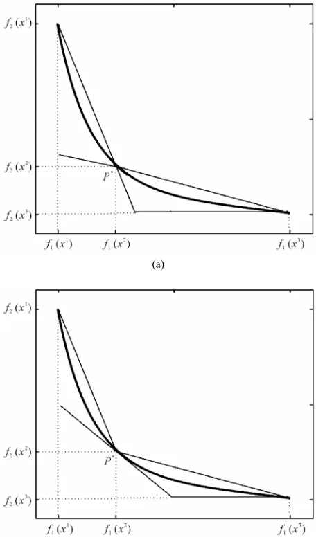
[image:5.595.309.537.288.705.2]The geometric illustration of STA and TA is given in Figure 1 and Figure 2, respectively. In Figure 1(a), there is an illustration of an efficient frontier and the corresponding lower and upper bounds determined by three initial points
(a)
(b)
3 3
1 , 2 .
f x f x
1 , 2f x f x
1 1 2 2
1 , 2 , 1 , 2 ,
f x f x f x f x
Here one can observe that in the interval
1 1
the Hausdorff measure 1
H
is the greatest. It means that we have to introduce a new point
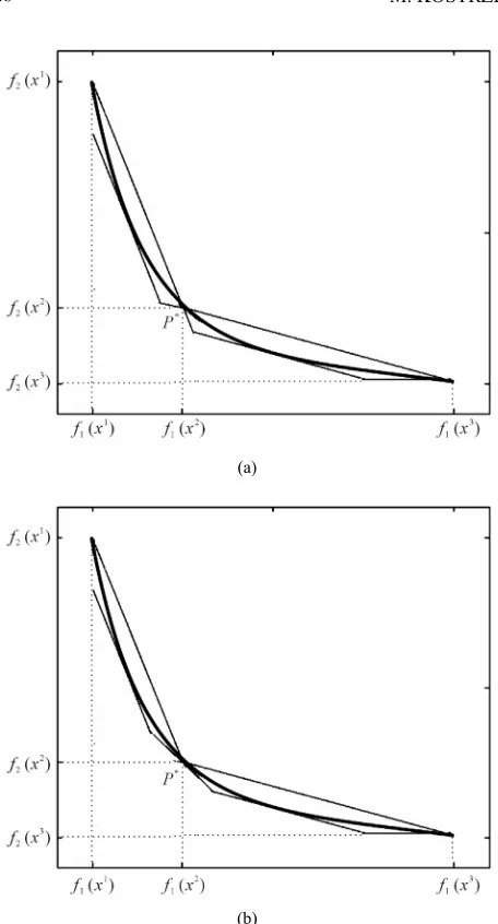
1 2 into the efficient frontier and determine new corresponding lower and upper bounds, what is illustrated in Figure 1(b). Similar considerations are illustrated in Figures 2(a) and 2(b).
x ,f x
P f
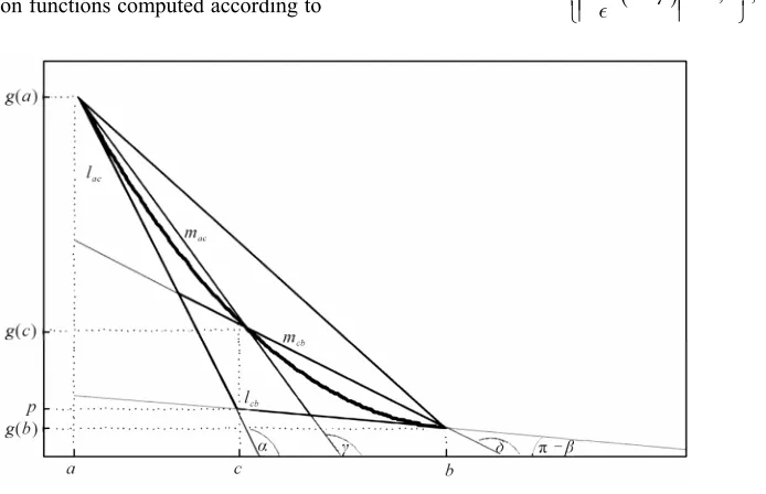
In Figure 3 and Figure 4 we see the illustration of STA and TA which lower bounds built due to definitions (9), (12) and (15), (19), respectively.
In Section 4 we study the convergence of described algorithms.
4. Convergence of the Algorithms
In this section we present the convergence results of presented algorithms based on proofs given in Rote [9]
(a)
[image:6.595.309.537.84.477.2](b)
Figure 2. Lower and upper bounds built due to TA.
(a)
(b)
Figure 3. Lower bounds in STA built due to definitions (9) and (12) presented in (a) and (b), respectively.
and Yang and Goh [8]. First, we formulate two following remarks, which show the relation between the considered error measures.
Remark 1
Suppose that the lower and upper approximation
11 , 1
k k
f x f x
have been bounds on the interval
build according to the definitions (8) and (9) or (15), then we have
2 1
2 2
1
1 1
1
k k
M H
k k k k
f x f x
f x f x
(31)
Moreover,
12 2
1
1 1
1
k k
M H
k k k k
f x f x
f x f x
(32)
See Figure 5.
[image:6.595.58.289.321.717.2](a)
[image:7.595.59.287.64.487.2](b)
Figure 4. Lower bounds in TA built due to definitions (15) and (19) presented in (a) and (b), respectively.
Remark 2
Suppose that the lower and upper approximation bounds on the interval
11 , 1
k k
f x
f x have been
build according to the definitions (8) and (9) or (15), then we have
2
21
2 .
k f xk
1
1 1 2
U H k k
k k f x f x f x
(33) Now, we suppose that the efficient frontier of problem (3) is given as a convex function g: a b
R and theone-sided derivatives g
a and g
b have beenevaluated.
[image:7.595.312.538.82.267.2]The following theorem based on Remark 3 and Theo- rem 1 in [8], Theorem 2 in [9] and Remark 1 and Remark 2 shows the quadratic convergence property of TA.
Figure 5. Illustration of error measures defined by (25)-(27).
Theorem 1
L ba and g
Let b g a and suppose
that the point
c g c,
was chosen to satisfy the fol- lowing inequality
.
b a
c a
g a g b
(34)
The number H of optimization problems (16) which
have to be solved in order to obtain the Hausdorff dis-tance between upper and lower bounds in TA smaller than or equal to satisfies the following inequality
max 2 L 1,3 .
H
(35)
The third point c g c,
,
L b a
on the efficient frontier has to be chosen if we want to avoid the problems with the leftmost interval in which theHausdorff distance between the approximation bounds is equal to the maximum error measure between them. The explanation how to determine a point with property (34) is given in the proof of Theorem 2.
Corollary 1
g
Let b g a
. The number M of
optimization problems (16) which have to be solved in order to obtain the Maximum error between upper and lower bounds in TA smaller than or equal to satisfies the following inequality
max 2 L 1 1,3 ,
M
(36)
g
where b g a . a b
The number U of optimization problems (16) which
C AJOR
a c, and
STA for interval c b,1
L L
, respectively, and and are the lengths of these intervals.
max 2
U L 1,3 ,
(37) 2
The next theorem based on Lemma 5, Theorem 2 from [9] and Lemma 3 establishes the linear convergence property of STA.
[image:8.595.58.219.86.145.2]where
2 a b 2.
g a g b
Theorem 2 Yang and Goh [8] noticed that the right directional de-
rivative
opyright © 2012 SciRes.
g a may be close to , that is why using
the fact that the Hausdorff distance is invariant under rotation it is better to consider the efficient frontier ro-
tated by π
4 with the modified directional derivatives
ag
and g
b and with L b a as the projec- [image:8.595.142.489.500.724.2]tive distance of the segment between points
a g a,
b g b,
and
onto the line m x
x.Also for STA we may find the upper bound for the number of optimization problems (16) or (28) which have to be solved. First, let us formulate the following lemma.
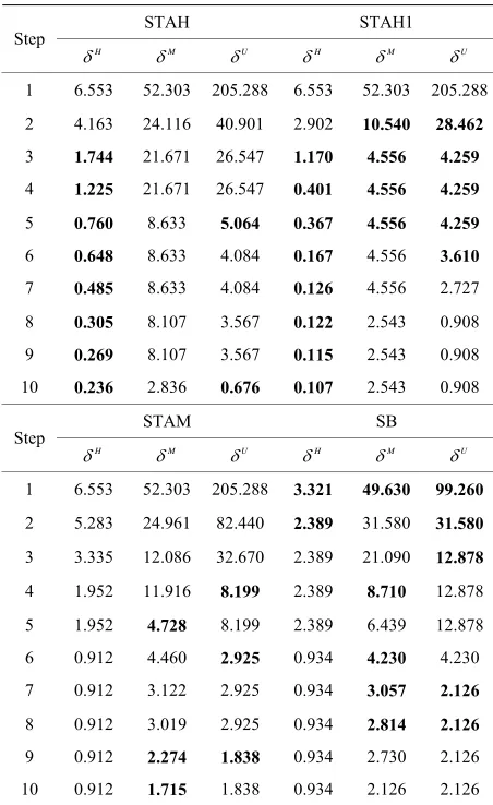
Lemma 3
Suppose that the convex function g: a b
R isapproximated from below by two linear functions lac
and lcb
such that lac
a g a
g b
ac
l c
cb
c a b
l b and
for some
cbl c
Let mac
andbe the lines which intersect the points
cb m
a g a,
,and , , respectively (see Figure 6
). If we denote byc c g c,
,c g
b g b,
tan, tan, tan, tan the slopes of lines lac
, lcb
, mac
, cb ,respec-tively, then the following inequality is satisfied
2 2 ,
L L L m
1 1
(38) where 1 tan tan , 2 tantan,
tan
tan
, L1 c a, L2 b c and L b a.
Proof: See Appendix.
Note that 1 and 2 are the differences of the slopes of lower approximation functions computed according to
Let
a g a,
,
c g c,
and
b g b,
are three ini-tial points which are necessary to start STA and suppose that
c g c,
was chosen to satisfy the following ine- quality
.
b a
c a
g a g b
L b a
(39)
and let g
Let a
, then the number
H of convex optimization problems ((16) or (28)), which
have to be solved in order to make the Hausdorff dis- tance between upper and lower bound in STA with the chord rule or the maximum error rule smaller than or equal to satisfies the following inequality
max L 4, 0
H .
(40) Proof: See Appendix.
Corollary 2
Let
a g a,
,
c g c,
and
b g b,
are three ini-tial points that are necessary to start STA and suppose that
c g c,
L b a
was chosen to satisfy the inequality (39). Let and let g
a
. The number M of
optimization problems (16) which have to be solved in order to obtain the Maximum error between upper and lower bounds in TA smaller than or equal to satisfies the following inequality
max L 1 4,0 ,
M
(41)
where g b
g a
. a b
The number U of optimization s (16) which hav
problem e to be solved in order to obtain the Uncertainty area error between upper and lower bounds in TA smaller than or equal to satisfies the following inequality
max L
U 4,0 ,
(42)
where
2 a b 2 . ark 3theorem is true for every convex func-
g a g b
Rem
Note that this
tion g:
a b R such that the one-sided derivative
g a valuated. If we do not have the deriva-
t formation using TA with maximum error rule gives us the linear convergence property of this proce- dure.
The following theorem by Rote [9] establishes the qu
has been e n
ive i
adratic convergence property of STA with the modi- fied lower bound as in (12).
Theorem 3
Let
a g a,
,
c g c,
and
b g b,
are three ini-ich a start ST
tial points wh re necessary to A and suppose that
c g c,
was chosen to satisfy the following ine- quality
b a .c a
g a g b
(43)
Let
L b a and let g a , then the number
nve problems (1
H of co imization 6), which have to
be solved in order to make the Hausdorff distance be-tween upper and lower bound in STA and TA with the modified lower bounds and the chord rule smaller than or equal to satisfies the following inequality
x opt
max 2,0 .
H
(44)
5. Examples
e define the stochastic minimum cost
at the
L
In this section w
flow problem with the moment bicriterion and present two numerical examples, which illustrate algorithm pre- sented in Section 3. Similar to the classic bicriteria net- work cost flow problem, we consider the directed net- work G with n nodes and m arcs with the node-arc inci-
dence matrix n m
DR , the net outflow vector bRn
and the capaci s , m.
l u
c c R Suppose th
cost per unit of flow thro rc i
1, , m
isdescribed by the random variable Ci R
ty bound
ugh the a
as-
sume that each variable Ci has positive expected value
and
i i
E C c and let C b a random vector such that
T
min T , , T
E x E f x
e stochast 1
C C, ,Cm . The ic minimum cost flow
problem with the moment bicriterion (SMCFP) is defined as follows
s t ,
,
l u
Dx b
c x c
C C
(45)
where : m m
f R R R is the continuous fu
that
nction such
, : mf a R R is convex for every aRm.
Since T
xE C x and x E f C x
,
are linearx functions, re
ind that the effic m (45 a
co rve in 2
R
and conve spectively, then using Lemma 1 we f ient frontier of proble ) is
nvex cu
e S
T T
The following two examples include the comparison of the results obtained by STA, TA with Yang and Goh’s method [8] and th iem et al.’s algorithm [7].
Example 1
We consider the simple stochastic minimum cost flow problem
minEC x,f x (46)
s.t.
1 2
4 5 1 2
1 3 4 2 3 5 4 5
2 6, 2 6, 0 4,
2 6, 2 6,
, , 8,
x x x
x x x
x x x x x x x x
3
8, x
where E C
1 3, E C
2 6, E C
3 1, E C
4 4,
5 2E C and
5 2
1 4
6 5
2 2
x
3
x
x x
x
f x e e e e e (47
The ve
)
ctors
6, 2, 4, 2,6
and 3
2,6,0, 2,6
x
are the lexicographical minima due to the f second criterion of problem (46) and
1
x
irst and the
1 1
1 1 , 2 54,82.12
P f x f x
and
3 3
3 1 , 2 62,12.47
P f x f x
o these vectors points on the efficient frontier. To avoid the problem with the leftm st interval we have taken
are corresponding t
o
2 54.15,74.63
P to be the third point
s algorithm (YG)
of the efficient frontier necessary to start STA and TA. The results’ comparison of subsequent calls of TA and Yang and Goh’ and the values of the Uncertainty area measure U after each step of TA
with the lower bounds defined in (19) (TA1) are pre- sented in Table 1. The results of STA, when new points are computed according to th maximum error rule in common with the Maximum error measure (STAM) and when new points are computed according to the chord rule in common with the Hausdorff measure with the lower bounds defined by the Equation (9) (STAH) and
Table 1. The results of subsequent calls of TA and Yang and Goh’s method (YG) for the problem described in example 1.
TA YG
Step H M U U (TA1)
H
M U
1 2.995 23.905 93.828 93.828 23.905 23.905 180.927
2 1.376 9.638 25. 23.644 5.308 9. 31.003
0.50 9.638 23.591 1.497 9.63 16.269
659 638
3 5 18.781 8
4 0.490 2.069 3.211 2.975 1.876 2.069 3.731
5 0.251 2.069 3.134 2.641 1.876 2.069 3.428
6 0.152 2.069 2.805 2.641 1.876 2.069 2.398
7 0.133 2.069 2.746 2.114 0.397 2.069 1.295
8 0.096 2.069 2.746 2.114 0.397 2.069 1.295
9 0.070 2.069 0.402 0.371 0.397 2.069 1.295
10 0.064 2.069 0.402 0.371 0.397 2.069 1.295
Table 2. re se
ch r T T e rr e
(STAM S l w t b n
le (SB) for the problem described in example 1. The
ule (S
sults of sub AH, S
quent c and th
alls of STA w maxim
ith the or rul
ord AH1) um e
) and iem e al.’s method ith in erval isectio ru
STAH STAH1 Step
H
M U H M U
(12) (ST are summ e
Ya an ’s od m ed e
inter als set eakpo nd -
bl in also the re h sc n
of the flo e network and the second moment of total co
,
l u
c x c
1 6.553 52.303 205.288 6.553 52.303 205.288
2 4.163 40.901 2.902 28.462
1.74 21.671 26.547 1.17 4.55 4.25 24.116 10.540
3 4 0 6 9
4 1.225 21.671 26.547 0.401 4.556 4.259
5 0.760 8.633 5.064 0.367 4.556 4.259
6 0.648 8.633 4.084 0.167 4.556 3.610
7 0.485 8.633 4.084 0.126 4.556 2.727
8 0.305 8.107 3.567 0.122 2.543 0.908
9 0.269 8.107 3.567 0.115 2.543 0.908
10 0.236 2.836 0.676 0.107 2.543 0.908
STAM SB Step
H
M U H M U
1 6.553 52.303 205.288 3.321 49.630 99.260
2 5.283 82.440 2.389 3 31.580
3.335 12.086 32.670 2.389 21.090 12.878 24.961 1.580
3
4 1.952 11.916 8.199 2.389 8.710 12.878
5 1.952 4.728 8.199 2.389 6.439 12.878
6 0.912 4.460 2.925 0.934 4.230 4.230
7 0.912 3.122 2.925 0.934 3.057 2.126
8 0.912 3.019 2.925 0.934 2.814 2.126
9 0.912 2.274 1.838 0.934 2.730 2.126
10 0.912 1.715 1.838 0.934 2.126 2.126
AH1) arized in Table 2. In th case of ng d Goh meth the errors are easur in th
v e 2
by th cludes
e br ints of sults of
the up the met
per bou od de
. Ta ribed i [7], which uses the interval bisection method of the computing new points with the Maximum error measure. After each step of algorithm we present the maximum values of three error measures: the Maximum error, the Hausdorff distance and the Uncertainty area. As we can notice TA and TA1 performs better than other algorithms giving in each step the smallest values of the Hausdorff distance measure and the Uncertainty area measure. Moreover, from Table 2 we can conclude that STA with the chord rule and the Hausdorff distance gives smaller values of the Hausdorff measure in each step than to two other algorithms, which give comparable results.
Example 2
We consider the stochastic minimum cost flow prob- lem in the network with 12 nodes and 17 arcs. We would like to minimize the mean value of the total cost
w through th
st, that is we solve the following problem
2min ,
s t ,
T
T T
E x E x
Dx b
C C
(48)
where 12 17
DR , bT
10,0, ,0, 10
, cT
0, ,0
and
l
6,6, ,6,6
T u
c and C
C1, , C17
T: R17is the random cost vector such that Ci and
j
C are
y independent for all i j, A such that i j.
mutuall
We have chosen the values of E C
1 , , E C17 from ntervalthe i
0, 2 and the values of the second mo-ments 2 2
1 , , 17
E C E C from the interval
1,3 Thepoints on the efficient frontier co e lexi-cographical m a of problem (48) and the second
cri-. rresponding to th inim
re
terion a P1 62.244, 6072.87 and
5.293,5145.63
. In thto STA and Siem e ethod. Table 3
includes the comparis 2
Yang and Goh’s method are considered, since from Ex- ample 1. follows that these two algorithms work faster in
comparison t al.’s m
on of TA with the method pre- sented in [8]. After each step of the considered methods we present the values of Hausdorff distance, Maximum error and Uncertainty area measure and a new evaluated point. As we can notice TA performs better in compare- son to Yang and Goh’s algorithm giving in each step the smallest value of the Hausdorff distance between upper and lower approximation bounds.
6. Conclusions
Two sandwich algorithms (the Simple Triangle Algorithm 6
P is example only TA and the
[image:10.595.58.284.364.733.2]alls of TA and Yang and G
TA YG
Table 3. The results of subsequent c oh’s method (YG) for the problem described in example 2.
Step
f x1
, 2
f x
H
M U H M U
1 1.507 458.259 1052.1 1.507 458.259 1397.42
2 (63.410, 5259.94) 0.59 117.1 36.287 117.1 129.2
(64.194, 176.09)
8 96 75.559 96 46
3 5 0.282 117.196 70.439 14.101 117.196 126.457
4 (64.733, 5153.34) 0.168 117.196 68.847 14.101 117.196 126.457
5 (62.824, 5551.23) 0.141 29.355 8.614 28.735 29.355 17.012
6 (65.013, 5147.54) 0.134 29.355 8.541 28.735 29.355 17.012
7 (63.584, 5227.26) 0.071 29.355 8.541 28.735 29.355 17.012
8 (65.1528, 5146.1) 0.058 29.355 8.534 28.735 29.355 17.012
9 (63.112, 5379.36) 0.053 29.355 8.523 7.254 29.355 15.961
10 (64.438, 5163.53) 0.042 29.355 8.523 7.254 29.355 15.961
and rap m) for proxim f
the cient gener bicriter -
um cost flow problem have been described. Both the T ezium Algorith the ap ation o effi frontier of the alized ia mini m
methods have been applied in the field of the stochastic minimum cost flow problem with the moment bicrite- rion.
The Simple Triangle Algorithm uses the lower bound proposed by Siem et al. in [7] with the maximum error
rule or the chord rule, what causes faster decrease of the Maximum error measure and the Hausdorff distance measure and, as a result, reduces the number of steps of algorithm in comparison to the Siem et al.’s method. We
have established the linear convergence property of this algorithm with both partition rules. If the lower bound in the Simple Triangle Algorithm is defined as in [9], ac- cording to the definition (12) and new points of the ef- ficient frontier are computed due to the chord rule then we have the quadratic convergence property of the algo- rithm.
From the numerical examples follows that the Trape- zium Algorithm performs better in comparison to all of the mentioned derivative free algorithms (Siem et al.’s
method, Yang and Goh’s method) and gives in each step the smallest values of the Hausdorff distance measure between lower and upper bound. It also works faster than Rote’s triangle algorithm. Moreover, Trapezium Algo- rithm may be used for approximation of any convex function without the assumption that the change of the direction of the tangents of this function is less than or
equal to π
2, see [8]. The quadratic convergence property of the Trapezium Algorithm has been established.
For further research we are interested in the construc-
tio method g the stic min flo blem with the moment iterion.
nal of
n of a for solvin stocha imum cost
w pro multicr
REFERENCES
[1] A. Sedeno-Noda and C. Gonzalez-Martin, “The Biobjec-tive Minimum Cost Flow Problem,” European Jour Operational Research, Vol. 124, No. 3, 2000, pp. 591- 600. doi:10.1016/S0377-2217(99)00191-5
[2] X. Q. Yang and C. J. Goh, “Analytic Efficient Solution Set for Multi-Criteria Quadratic Programs,” European Journal of Op l. 92, No. 1, 1996, pp. 166-181. doi:10.1016/0377-2217(9erational Research, Vo5)00040-2
[3] G. Ruhe, “Complexity Results for Multicriterial and Pa-rametric Network Flows Using a Pathological Graph of Zadeh,” Zeitschrift für Operations Research, Vol. 32, No. 1, 1988, pp. 9-27. doi:10.1007/BF01920568
[4] N. Zadeh, “A Bad Network for the Simplex Method and Other Minimum Cost Flow Algorithms,” Mathematical Programming, Vol. 5, No. 1, 1973, pp. 255-266.
doi:10.1007/BF01580132
[5] R. E. Burkard, H. W. Hamacher and G. Rote, “Sandwich Approximation of Univariate Convex Functions with an Applications to Separable Convex Programming,” Naval Research Logistics, Vol. 38, 1991, pp. 911-924.
nal of . 42, No. 3, 1989, pp. 326-338. [6] B. Fruhwirth, R. E. Burkard and G. Rote, “Approxima- tion of Convex Curves with Application to the Bi-Criteria Minimum Cost Flow Problem,” European Jour Operational Research, Vol
doi:10.1016/0377-2217(89)90443-8
[7] A. Y. D. Siem, D. den Hertog and A. L. Hoffmann, “A Method for Approximating Univariate Convex Functions Using Only Function Value Evaluations,” Center Dis- [8] X. Q. Yang and C. J. Goh, “A Method for Convex Curve
Approximation,” European Journal of Operational Re- search, Vol. 97, No. 1, 1997, pp. 205-212.
doi:10.1016/0377-2217(95)00368-1 [9] G. Rote, “The Convergence Rate of th
rithm for Approximating Convex Functions,” Computing, Vol. 48, No. 3-4, 1992, pp. 337-361.
doi:10.1007/BF02238642 e Sandwich