Seeing Through the Fog: Using Scattered Light to Peer Deeper into Biological Tissue

(1)

Using Scattered Light to Peer Deeper into Biological

Tissue

Thesis by

Joshua Harris Brake

In Partial Fulfillment of the Requirements for the Degree of

Doctor of Philosophy

CALIFORNIA INSTITUTE OF TECHNOLOGY Pasadena, California

2019

(2)

Joshua Harris Brake ORCID: 0000-0002-5113-6886

(3)

ACKNOWLEDGEMENTS

"If I have seen further it is by standing on the shoulders of giants." - Isaac Newton

During the course of my PhD studies at Caltech there are numerous people who have made a significant impact not only on my development as an engineer and scientist, but also as a person. I am very thankful for all those who have poured into me, and hope that I can model the lessons they have taught me as I seek to mentor and guide the next generation of budding scientists and engineers.

First of all, I am grateful to my advisor Prof. Changhuei Yang for seeing something in me when I applied, and mentoring me over the past five years. He is an encouraging and honest advisor who has been a constant support during my PhD journey. I am thankful for his critiques and suggestions about my research ideas and his financial support for my studies, research supplies, and conference travel. I continue to appreciate the way he tailors his guidance to the individual needs of the members in the group and the energy he brings to the field of biophotonics.

(4)

Xiaoze Ou, Daifa Wang, Donghun Ryu, Liheng Bian, Yidong Tan, Helen Lu, Daniel Martin, Yujia Huang, Michelle Cua, Cheng Shen, Changsoon Choi, Ruizhi Cao, and Antony Chan. Finally, a big thanks to Anne Sullivan for all her help over the years with ordering and helping keep the group operations running smoothly.

I would also like to thank my committee members Prof. Lihong Wang, Prof. Viviana Gradinaru, Prof. Azita Emami, and Prof. Euiheon Chung. It is a privilege to have the opportunity to work with such world-class scientists and engineers and to learn from their critiques and suggestions.

My life outside the lab in Pasadena over the past five years has also been a rich one and has helped me to bring a fresh and resilient attitude to the lab. In particular I am thankful for the great church home Abbey and I found at Grace Pasadena. The entire church staff made us feel welcome from our first week visiting and has helped both Abbey and I feel at home in Pasadena. For that I am thankful; especially to Brannin and Tanya Pitre, Marc Choi, and Jen Argue. I am also especially thankful for my friend Ben Ewen who has been an encouragement to me throughout my studies (and for his contributions to my coffee hobby!). Our city group has been a source of encouragement each week, and I have been enriched by the fellowship each Friday morning with the Grace men’s group (Ben Ewen, Dave McFadzean, Justin Su, Eric Branscum, Mark Pickett, Zach Lee, and Gene Fahnestock). I have also been blessed to work alongside Len Tang and Jeff Still to launch the Science and Faith Examined project on the Caltech campus and have been blown away by how God has used it to spark conversations, develop relationships, and open doors for the Gospel on campus.

(5)

There are many past teachers from my undergrad years at LeTourneau University that were integral in getting me to where I am today. I will always be thankful for Bill Graff and the many lessons I learned both as his student and from my experience getting to teach alongside him. My pedagogical approach has been shaped by the concepts I saw him use like frequent low-stakes testing and hands-on active learning with lab exercises. I am also thankful for others at LeTourneau like Paul Leiffer and Joonwan Kim and the lessons they taught me about how to live as a faithful Christian engineer. Others who had an impact during my student years include my research advisor Seung Kim and thesis advisor Steve Ball.

I also owe thanks to several instrumental high-school teachers: Dan Vinton for teaching me to love math early on, and Jim Bair for helping me hone my writing and always ask "so what?"

Throughout my life, I am particularly thankful for the support, encouragement, example, and love of my family. My grandparents Roger and Eleanor Brake and Gordon and Bernina Danielson always supported and encouraged me. My grandfa-ther Roger Brake, in particular, taught me the value of not only working hard, but working smart.

I am also deeply indebted to my parents Jim and Marjie Brake. Mom, I’ll always remember the homeschool days, and all the hours you spent teaching Nate and me and helping with a variety of school-related activities throughout elementary and high school. Dad, for your example of working hard, managing what the Lord has given you well, and faithfully providing for your wife and kids. I’m also thankful for my brother Nate and sister Rachel and their encouragement and support over the years.

Abbey, I am so grateful to have had you at my side for these past 5 years as my wife (not to mention the many years prior as my best friend) and to be experiencing life together with you day by day. I cannot wait to see what the Lord has for us and our family in this next stage at Harvey Mudd. I love you.

(6)

(7)

ABSTRACT

Optical scattering is a fundamental problem in biomedical optics and limits most optical techniques to shallow operating depths less than 1 mm. However, although the scattering behavior of tissue scrambles the information it contains, it does not destroy it. Therefore, if you can unscramble the scattered light, it increases the accessible imaging depths up the absorption limit of light (several centimeters deep).

One such way to beat optical scattering is using wavefront shaping. Borrowing ideas from adaptive optics in astronomy and phased arrays in radar and ultrasonic imaging, the basic concept of wavefront shaping is to control the phase and amplitude of the light field in order to harness scattered light. Using wavefront shaping techniques, scattered light can be used to form focal spots or transmit information through or inside optically scattering media. Furthermore, even without correcting for scattering directly by shaping the input light field, the properties of the scattered light can be analyzed to recover information about the structure and dynamic properties of a sample using methods from diffuse optics.

The main contributions of this thesis are along these two lines of research: moving wavefront shaping toward more practical applications and developing new tech-niques to recover useful physiological information from scattered light. This is developed through three main projects:

1. An investigation of how dynamic samples impact the scattering process and the practical implications of these dynamics on wavefront shaping systems.

2. The development of a wavefront shaping system combining light and ultra-sound to focus light inside acute brain slices to improve light delivery for optogenetics.

(8)

PUBLISHED CONTENT AND CONTRIBUTIONS

• D. Wang†, E. H. Zhou†,J. Brake, H. Ruan, M. Jang, and C. Yang, “Focusing through dynamic tissue with millisecond digital optical phase conjugation,” Optica, 2(8), pp. 728–735, 2015. DOI: 10.1364/OPTICA.2.000728

J. B. helped prepare the some of the figures and develop the flow and presen-tation of the results in the manuscript.

• J. Brake†, M. Jang†, and C. Yang, “Analyzing the relationship between decor-relation time and tissue thickness in acute rat brain slices using multispeckle diffusing wave spectroscopy,” JOSA A, 33(2), pp. 270–275, 2016. DOI: 10.1364/JOSAA.33.000270

J. B. developed the experimental setup with help from M. J., drew the figures, and wrote and edited the manuscript with help from M. J. and C. Y.

• E. H. Zhou, A. Shibukawa, J. Brake, H. Ruan, and C. Yang, “Glare sup-pression by coherence gated negation,”Optica, 3(10), pp. 1107–1113, 2016. DOI: 10.1364/OPTICA.3.001107

J. B. helped design the figures, develop the data visualization, and write the manuscript.

• M. M. Qureshi†, J. Brake†, H.-J. Jeon, H. Ruan, Y. Liu, A. M. Safi, T. J. Eom, C. Yang, and E. Chung, “In vivo study of optical speckle decorrelation time across depths in the mouse brain,” Biomedical Optics Express, 8(11), pp. 4855–4864, 2017. DOI: 10.1364/BOE.8.004855

J. B. helped to design the experiment with M. M. Q., analyzed the data, drew the figures, and helped write the manuscript.

• H. Ruan†, J. Brake†, J. E. Robinson, Y. Liu, M. Jang, C. Xiao, C. Zhou, V. Gradinaru, and C. Yang, “Deep tissue optical focusing and optogenetic mod-ulation with time-reversed ultrasonically encoded light,” Science Advances, 3(12), eaao5520, 2017. DOI: 10.1126/sciadv.aao5520

(9)

• H. Ruan, T. Haber, Y. Liu, J. Brake, J. Kim, J. M. Berlin, and C. Yang, “Focusing light inside scattering media with magnetic-particle-guided wave-front shaping,” Optica, 4(11), pp. 1337–1343, 2017. DOI: 10.1364/OP-TICA.4.001337

J. B. helped to develop the experimental procedure and to prepare and edit the manuscript.

• M. Jang†, Y. Horie†, A. Shibukawa†, J. Brake, Y. Liu, S. M. Kamali, A. Arbabi, H.Ruan, A. Faraon, and C. Yang, “Wavefront shaping with disorder-engineered metasurfaces,” Nature Photonics, 12(2), p. 84, 2018. DOI: 10.1038/s41566-017-0078-z

J.B. helped develop the idea, draw the figures, and write and edit the manuscript.

(10)

LIST OF ILLUSTRATIONS

Number Page

1.1 Jablonski diagram . . . 3

1.2 Scattering on a foggy morning in Pasadena, CA . . . 4

1.3 Scattering through thick slab of scattering material . . . 6

1.4 Cartoon describing how the directionality of scattered light is quantified. 7 1.5 A cartoon describing the principle of temporal coherence. . . 12

1.6 A cartoon describing the principle of spatial coherence . . . 14

1.7 Simple holography schemes. . . 16

1.8 Shot noise explanation with a raincloud and showerhead . . . 20

1.9 Scattering regimes . . . 23

1.10 Transmission matrix diagram . . . 25

1.11 Phasor diagram illustrating the interference of different modes in a speckle pattern. . . 28

1.12 Feedback-based wavefront shaping . . . 30

1.13 Time-reversal-based wavefront shaping . . . 31

2.1 Experimental setup used to capture the speckle patterns. . . 40

2.2 g2(τ)decorrelation time calculation . . . 41

2.3 Decorrelation curves for 1.0, 1.5, 2.0, and 3.0 mm thick brain slices. . 42

2.4 Decorrelation times of the individual trials plotted with respect to tissue thickness. . . 43

2.5 Results of the Monte Carlo simulation of 1×106photons with tissue properties µs = 5/mm, µa= 0.2/mm, andg= 0.9. . . 45

2.6 Inverse mean path lengthhP(s)ivs sample thickness from 1-3 mm. . 46

3.1 Diagram of the experimental setup . . . 55

3.2 Characterization of diffusing fiber tip light distribution . . . 56

3.3 Decorrelation curves for different fiber tip depths . . . 58

3.4 Decorrelation time as a function of fiber tip penetration depth . . . . 59

4.1 Custom TRUE focusing and electrophysiological recording system . . 69

4.2 Schematic of the TRUE focusing system . . . 70

4.3 TRUE Focusing system electrical signal flow diagram . . . 71

(13)

4.5 Experiment design, opsin characterization, and demonstration of

photocurrent and firing modulation via TRUE focusing . . . 76

4.6 Ultrasound pulse-echo image of the tip of the glass pipette electrode . 78 4.7 Electrophysiological photocurrent traces from neurons in 500 µm and 300 µm thick acute brain slices . . . 79

4.8 Electrophysiological photocurrent and membrane voltage traces com-paring ultrasound on and off conditions . . . 80

4.9 Spatial resolution of optogenetic stimulation achieved by conven-tional versus TRUE focusing . . . 81

5.1 iSVS decorrelation explanation . . . 96

5.2 iSVS data processing procedure . . . 98

5.3 iSVS Experimental Setup . . . 100

5.4 Advantage of vertical slit in the Fourier domain for optimal spatial frequency bandwidth usage . . . 101

5.5 Rotating diffuser calibration setup . . . 102

5.6 iSVS and SVS results vs. decorrelation time with rotating diffuser . . 102

5.7 iSVS and SVS results in the dorsal skin flap: transmission . . . 104

(14)

C h a p t e r 1

INTRODUCTION

“If you see through everything, then everything is transparent. But a wholly trans-parent world is an invisible world. To ‘see through’ all things is the same as not to see.” - C.S. Lewis

Focusing light into biological tissue is a critical capability in medicine, for a variety of diagnostic and research purposes. Medical imaging technologies using magnetic resonance, ultrasound, X-ray, or positron emission can penetrate deeply through tissue and thus enable entire organisms or parts of organisms to be imaged. However, each of these imaging technologies suffers from drawbacks, which prevent them from being maximally useful for biological diagnostic imaging or sensing. For example, the large magnetic fields necessary for magnetic resonance imaging (MRI) make it challenging to design affordable and compact systems. Furthermore, the resolution of MRI typically cannot extend beyond a cubic millimeter, which limits the ability to examine the fine structural or functional signals that are of interest in the brain as measured in functional MRI. Ultrasound, while noninvasive and safe even for the most delicate of tasks such as imaging babies in the womb, has limited spatial resolution due to the size of the acoustic wavelengths used and often needs additional contrast mechanisms to enable high enough signal-to-noise ratio (SNR) to image the structures of interest. Finally, X-ray and positron emission tomography use ionizing radiation, which can damage the sample under examination and are also limited in terms of the types of contrast they can image.

(15)

the physical and mathematical origins of optical imaging and strategies to address this scattering.

1.1 Light-Matter Interactions

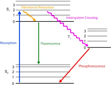
The many types of interaction between light and matter provide a wide range of different contrast mechanisms that can be used to interrogate samples of interest. In optics, these contrast mechanisms can be exploited in order to provide information about the structure and function of different materials inside the medium. The foundation for light matter interaction is based on the electronic structure of the atoms and molecules making up the matter. Molecular and atomic energy levels exist are quantized and the distribution and spacing between these levels specify their electronic behavior. The Jablonski diagram is a visual representation of this electronic structure and is helpful for discussing light matter interactions. An example of a Jablonski diagram is shown in Figure 1.1. The thick solid lines indicate the electronic states and the thinner lines indicate different vibrational states within the given electronic states. Nonradiative transitions are indicated by straight arrows while radiative transitions are indicated by squiggly lines. These different types of transitions will be described subsequently.

In general, there are two main classes of light-matter interaction, resonant and non-resonant. These classes provide the physical basis for contrast mechanisms such as absorption, fluorescence, phosphorescence, and scattering.

Resonant interactions refer to those where the energy of the incoming photon matches one of the internal energy levels present within the atomic structure of the material. When this matching occurs, the molecule can absorb the energy from the incoming photon and cause an electron to jump to an excited state. When the molecule is in the excited state, it will naturally relax to a lower energy state. This decay can happen through two main pathways: nonradiative and radiative relaxation.

(16)

[image:16.612.126.487.80.363.2]

Figure 1.1: An example of a Jablonski diagram.

on a much slower time scale, from 10−8to 10−3seconds.

Raditive processes are those in which a photon is reemitted as the excited electron decays to a lower energy state. Fluorescence is the process by which electrons relax from an excited electronic state to a lower electronic energy level and emit a photon. The electron maintains its spin state, and so this is a relatively fast process, typically ranging from one to one hundred nanoseconds. In contrast, phosphorescence occurs when the excited electron relaxes but changes its spin state. Since this process requires an intersystem crossing, it has a much slower time scale than fluorescence, typically ranging from the millisecond range to several seconds.

(17)

[image:17.612.112.500.72.298.2]

Figure 1.2: Scattering on a foggy morning in Pasadena, CA.

incoming photons. Nonresonant interactions also include scattering phenomena such as Raman scattering. While this is an inelastic scattering mechanism since the energy of the emitted light differs from that of the incident light, it is distinct from the resonant interactions since the energy states of interest are virtual states, not actual energy levels that exist within the electronic structure of the molecules.

These light-matter interactions are what enable imaging systems, whether cameras or the human eye, to form images of the world around us. Light as it illuminates an object encounters the boundary of the object which causes it to be absorbed, reflect, or refract based on the optical properties of the interface (e.g., the absorptivity or the change in refractive index). Scattering from differences in refractive index is fundamental to imaging since it causes the light to be redirected, enabling it to be captured by an imaging system. However, while the scattering of light is an important form of optical contrast, enabling us to be able to see anything at all, unwanted scattering (or more precisely uncontrolled scattering as we will see later in thesis) is detrimental in an optical system.

(18)

the optical opacity of clouds as the sun tries to pierce through them on an overcast day. From the perspective of microscopy, the unwanted scattering of rough tissue interfaces or out-of-focus layers within a biological tissue sample scatter light and prevent clear imaging of the deeper layers below. For this reason, most biolog-ical tissue samples used in microscopy are cut in thin slices to limit the degree of unwanted scattering. Unfortunately, cutting the samples into thin slices creates additional levels of complexity and has undesirable side effects such as physically damaging the sample and making three-dimensional registration of the components within the tissue difficult.

In the next sections, we will look in more detail about how we can mathematically describe the physical phenomena of light scattering and absorption and build models to inform the development of optical tools for biomedicine.

Light Scattering Modeling Scattering Coefficient Derivation

To get a better understanding of elastic scattering, it is helpful to spend a few para-graphs to develop a simple mathematical model to describe the scattering process. This model will allow us to build up from first principles an intuitive mathematical understanding of how we can visualize scattering and provide us with several quanti-tative measures of optical scattering (such as the strength of scattering, directionality of scattering, and the delineation different scattering regimes).

In this section, quantities will be given names with their dimensions in square brackets (e.g., a distance x has a dimension of length denoted by[l]). To start, we will consider the transmission of light through a sample of thickness L[l] with a number volumetric concentrationn#·l−3 of scatters with scattering cross-section

σs

l2

. Now, using a typical trick in calculus, we will slice our thick scattering medium of thickness L into an arbitrarily small thickness δx[l]. The number of scatterers in this slab isnAδx[#].

Now for this slab, what is the probability that a photon will pass through the slab unscattered? First, we can derive probability that a photon is scattered which is simply given by

P(_scatteredδx)= Ratio of scattering area Total area of slab =

(nAδx)σ_s

(19)

Figure 1.3: Scattering through thick slab of scattering material. (a) A scattering medium of cross-sectional area A and thickness L. (b) A slice of the scattering medium of thicknessδx.

From this, we can calculate the probability that a photon is unscattered as

P(_unscattered_δ_x)=₁−P(_scattered_δ_x)=₁−nδxσs = exp(−nδxσs) (1.2)

where the last step uses the fact that δx can be made arbitrarily small to use the Taylor series expansion to represent the probability as an exponential.

This allows us to calculate the probability of a photon passing through the whole slab unscattered as the probability that it passes through a succession of individual thin slabs with the probabilities of being unscattered as given in Eq. 1.2. By definition, the number of slabs that makes us our whole scattering sample is given by _δL_x [#]. So, the probability of a photon passing unscattered through the entire slab is given by

P(_unscatteredL)= _exp(−nδxσs) L

δx =_exp(−_nσ

sL). (1.3)

This leads to the definition of a dimension of interest for scattering, the scattering mean free pathls[l]or its inverse, the scattering coefficientµs = nσs

l−1

. Formally defined, this is the thickness at which the fraction of unscattered light is given by 1_e.

Scattering Anisotropy

(20)

How-Figure 1.4: Cartoon describing how the directionality of scattered light is

quan-tified. (a) An incident collimated beam is incident on a scattering medium such as a cell or piece of tissue. After interacting with the cell, the exiting light is scattered into different directions and can be quantified by measuring the intensity of light directed into a given angle. (b) A plot of scattered light intensity vs. angle for a solution of 1 µm spheres with refractive index ofn= 1.5 suspended in water (refrac-tive indexn= 1) illuminated with 532 nm light at a concentration of 0.1 spheres per cubic micron. Plots calculated using the Mie scattering calculator from the Oregon Medical Laser Center (OMLC) Mie Calculator.

ever, the degree to which light is redirected from the original propagation direction into another direction differs based on the physical parameters of the sample. We can quantify this directionality by measuring the intensity of the scattered light as a function of angular deviation from the original propagation direction as shown in Figure 1.4.

(21)

g =

∫ π

0

p(θ)_cos(θ)₂π_sin(θ)dθ = hcos(θ)i _(1.4)

The anisotropy factorggives a quick sense of the scattering behavior and describes how forward scattering a material is. When the scattering is in the forward direction, theng∈ (0,1]withg ≈1 representing strong forward-directed scattering, when it is isotropic theng =0, and when the scattering is backward directed theng ∈ (0,−1]. In biological tissue, which is in general very forward scattering, a typical value ofg is∼ 0.9.

The most important parameter governing the directionality of the scattered light is the size of particle compared to the wavelength of light. We can separate it into three general cases. When the particle is much smaller than the wavelength of light (d << λ/10), the scattering is nearly isotropic and g ≈ 0. This regime is called Rayleigh scattering. In this regime, the intensity of the scattered light scales according to inverse of the wavelength to the fourth power (Iscattered = λ

−₄

). Thus, in the Rayleigh regime, shorter wavelengths scatter much more strongly than longer ones. The most common everyday manifestation of Rayleigh scattering is the blue color of the sky.

When the size of the particle is on the same order as the wavelength, the anisotropy can vary quite drastically based on the size of the particle and the difference be-tween its refractive index and that of the background media. This regime can be described and analyzed using Mie theory and the Van de Hulst method. Finally, when the particle is much larger than the wavelength (d > 10λ), geometric optics can accurately describe the scattering phenomena. However, most of the interesting scattering in biomedicine is caused by particles on the order or smaller than the optical wavelength such as organelles and cell membranes.

Transport mean free path

(22)

A helpful rule of thumb for the length scale at which this diffusion process takes over is called the transport mean free path (l∗) and is defined as

l∗ = l

(₁−g). (1.5)

The transport mean free path represents the distance where effectively no ballistic photons remain and is the point at which conventional optical microscopy techniques that rely on ballistic light begin to fail. The typical transport mean free path in biological tissue isl∗ ≈1 mm.

Mie Theory and the Rayleigh-Gans-Debye Approximation

In a scattering medium like biological tissue, there are many scattering events and it is hard to usefully characterize the scattering behavior with anything but the parameters we have already discussed like mean free path, transport mean free path, anisotropy, etc. However, to get a better sense of how scattering happens, we can simplify the problem and look at the scattering due to a single spherical particle. Mie theory, developed by Gustav Mie, is an exact solution to Maxwell’s equations for the scattering behavior of a spherical particle under illumination by a electromagnetic plane wave. From Mie theory, we can better understand the specific behavior of scattering and then abstract this knowledge to more complicated cases.

In the case where the refractive index contrast of the sphere (i.e., the relative refractive index of the spherens compared to the background mediumnbis nearly 1,

ns nb −1

<< 1) and the phase shift of the light passing through the sphere is

small 2ka

ns nb −1

<< 1), an approximation known as the Rayleigh-Gans-Debye

approximation can be applied to simplify the Mie theory. Interested readers are suggested to consult reference [1] for more details.

Light Absorption

(23)

the energy that is now contained in the excited electron vibrations can either be transferred to another molecule, re-emitted as light at a lower energy, or emitted as heat.

Following a similar derivation as used above for scattering, we can also develop a metric to quantitatively describe the amount of absorption in a given medium. To start, we will again imagine a thick slab of material with a number concentration of absorbers given byn#·l−3 and an absorption cross section given byσa

l2_.

Again, dividing up the medium into thin slices of thicknessδx[l]we can calculate the probability of a photon not being absorbed as

P(_unabsorbed_δ_x)= ₁−P(_absorbed_δ_x)= ₁−nδxσa= exp(−nδxσa). (1.6)

Again, expanding this to the entire thickness L of the absorbing medium, we can find that the probability of a photon being unabsorbed is given by

P(_unabsorbed_L)=_exp(−nδxσa) L

δx =_exp₍₋_nσ

aL). (1.7)

Here, we see alignment with the Beer-Lambert law and we can define a characteristic lengthla[l](or equivalently the absorption coefficient µa

l−1_{) that describes the}

thickness of absorbing medium where the exiting power is equal 1_etimes the incident power.

1.2 Relevant Properties of Light

In addition to the properties which describe light-matter interaction, there are also several important properties of the light itself which we need to discuss. These include basic quantities such as wavelength, frequency, and energy as well as more advanced but nonetheless important properties such as coherence (spatial and tem-poral) and interference. In addition, after understanding these basic properties, we will more fully be able to understand the fundamental physics of different light sources and how they can be appropriately used in the development of optical tools.

(24)

length,νis the frequency with units of inverse time, andcis the speed of light with units of length per unit time.

λν=c (1.8)

The energy of light is also an important quantity. It as well is related to the frequency of the light and is given by

E = hν, (1.9)

whereEis the photon energy,his Planck’s constant with units of energy times time, andνwhich has units of inverse time.

Properties of light

More advanced properties of light are also important for describing the behavior of optical systems. One of these properties is coherence. Coherence has two main dimensions; temporal and spatial.

Temporal coherence

Temporal coherence describes the correlation of wave and a copy of itself delayed by a timeτ. Temporal coherence can be quantified either as a coherence timeτc, which is defined as the delay time after which the correlation drops below a specified value such as 1/e, or a coherence length, which is equal to the coherence time multiplied by the speed of light to convert it into a unit of length. Often, the coherence length is a more convenient quantity since it has more direct implications on the physical design of optical systems.

To intuitively understand the concept of temporal coherence, we can imagine two cases. If we have an idealized continuous wave, single frequency source, the coherence length will be infinite since the wave will always perfectly correlate with itself, regardless of the delay time/length. The interference patterns for this source will always have a very high contrast and will exhibit strong constructive and destructive interference depending on the exact values of the delay time. A laser is an example of a source that is typically designed to have a very long coherence length since it contains a very narrow range of emitted frequencies.

(25)

[image:25.612.121.485.134.423.2]

(26)

(LED)), this will yield a shorter coherence length. In this case, because the overall intensity of the resultant interference pattern is due to the summation of the individual frequencies, the resulting interference plot for different delay times is reduced. The reduction in correlation is directly determined by the spectral bandwidth (i.e., range of emitted frequencies) of the source. In addition to LEDs, short pulsed lasers are another type of light source that exhibits short coherence lengths. The operation of mode-locked lasers can make this connection particularly clear since the locked phase of different wavelengths causes the individual frequencies to phase in and out and create the resulting pulses.

Mathematically, we can describe the temporal coherence of a source using an autocorrelation function,G(τ), given by

G(τ)= hU∗(t)U(t+τ)i _(1.10)

whereU(t) is a stationary random complex optical wavefunction representing the light source and τ is a delay time. The temporal autocorrelation function can be normalized by its value at t = 0 which is equivalent to the overall intensity of the source. This yields the normalized autocorrelation function given by

g(τ)= hU

∗₍_t₎_U₍_t₊_τ_)i

hU∗(t)U(t)i . (1.11)

The value of |g(t)|indicates the complex degree of temporal coherence of a source where|g(τ)| = 1 indicates a perfectly correlated source and |g(τ)| = 0 for a totally uncorrelated source.

Spatial coherence

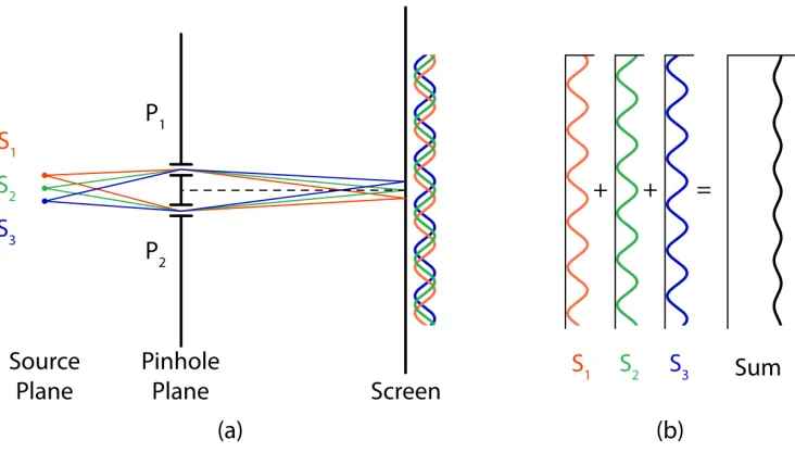
Spatial coherence refers to the phase correlation of a wavefront and can be understood to represent how closely the light source corresponds to an ideal point source. Consider the Huygens-Fresnel principle, which states that each point on a wavefront acts as a new source of spherical wavefronts and a Young’s double slit experiment. Assuming a temporal coherence length much longer than the path length difference between the light emitted from S1 and arriving at the screen from the two slits, we

expect to see an interference fringe pattern. S2 will contribute a similar, shifted

(27)

[image:27.612.120.486.76.290.2]

Figure 1.6: A cartoon describing the principle of spatial coherence. (a) Several sourcesS1, S2, andS3, illuminated two pinholesP1andP2. These sources generate

fringe patterns on the screen. The number of independent sources or equivalently the spatial extent of the resulting extended source determines the spatial coherence of the source. (b) Summing the shifted fringe patterns from each of the individual sources generates a reduced contrast fringe pattern.

The argument of how we arrive at spatially incoherent illumination is very similar to the argument we just followed to arrive at temporally incoherent illumination. In the case where we only have one point sourceS1emitting light, we end up with a

single fringe pattern, and if the source is a true point source (infinitely small) and the temporal coherence of the source is infinite (monochromatic), then the fringe pattern on the screen will be high contrast regardless of the separation distance of the pinholesP1andP2. If, however, we consider the addition of more point sources

S₂and S3, the situation will begin to change. This situation is illustrated in Figure

1.6(a) with the summation of the fringes and resulting reduction in fringe contrast shown in Figure 1.6(b).

(28)

the reader is encouraged to consult reference [2].

Source properties and applications

When designing an optical system, is it critical to carefully choose a source with the appropriate properties. For example, we generally want to avoid strong absorption from water and depending on the application, may want to carefully choose our wavelength(s) to measure the absorption of blood or excite a particular molecule within the tissue. In other imaging applications, we may want to minimize the overall absorption to be able to image deep inside tissue. The coherence properties are also critically important and in particular, the temporal coherence properties of a source can help to improve the resolution and isolate signal photons by using interference as in imaging strategies such as optical coherence tomography (OCT) [3].

1.3 Interferometry

One of the challenges of working with the optical portion of the electromagnetic spectrum is that the frequency is very high. The high frequency (several hundred terahertz) is faster than electronic circuits can operate and therefore, unlike lower frequency signals like microwave or radio frequency signals, optical measurements do not have direct access to the complex (amplitude and phase) information of optical signals. Instead, optical measurements are most commonly made of the optical intensity, the time-averaged magnitude squared of the complex field (I = |E|2, integrated over some measurement time. While the amplitude of the complex signal is simply the square root of the intensity |E| =

√

I, the phase information is lost.

Unfortunately, in many optical applications, the phase information is very important as it carries valuable information about the optical field.

(29)

detec-Figure 1.7: Simple holography schemes. (a) Phase shifting holography setup. The phase shifter (typically an electro-optic modulator (EOM) or delay line with translating mirror) is used to introduce phase shifts (optical path delays) between the sample and reference beams. (b) Off-axis holography setup. The reference beam is tilted by an angle of α with respect to the sample beam normal direction. This separates the sample and reference terms in the spatial frequency domain, enabling them to be retrieved from a single-shot measurement.

tors. The operation principles and respective trade-offs of these approaches will be described in the next sections.

Phase-shifting holography

(30)

I(x)=

∫

T

|E_s+E_r|2=

∫

T

EsEs∗+ErEr∗+EsEr∗+Es∗Er (1.12)

=∫

T E2

s +Er2+2EsErcos(φs(x−φr(x)) (1.13)

where the∗stand for complex conjugation.

We can see from this equation that the overall intensity is a function of the sample and reference intensities plus a term that contains the product of the sample amplitude, reference amplitude, and the cosine of the phase difference between the sample and reference beams. By changing the phase difference between the sample and reference beams, we can encode the phase difference information into the intensity. Normally, this is done by shifting the phase of the reference beam with respect to the sample beam with either a translating delay line or electro-optic modulator (EOM). By capturing at least three intensity measurements with different phase shifts, the phase of the sample beam can be reconstructed. For simplicity and signal to noise considerations, four different phase shift values are normally measured with relative phase difference ofθ ∈ [0, π/2, π,3π/2]. In this case, the phase of the sample beam can be recovered using the simple equation below.

φs =tan−1

I₃π/₂−Iπ/₂ Iπ−I₀

(1.14)

The drawbacks of the phase shifting holography method is that it requires at least three frames to measure the phase of the sample. However, it enables full use of all the pixels in an area detector, since the phase is measured at each pixel.

Off-axis holography

(31)

and θy are the tilt angles with respect to the x and y directions respectively. This yields an expression for the intensity given by

I(x)=

∫

T

|E_s+E_r|2=

∫

T

EsEs∗+ErEr∗+EsEr∗+Es∗Er (1.15)

=

∫

T E2

s +Er2+Ese

−jφs(x)_Er_ej k(sinθxx+sinθyy))+_Es_ejφs(x)_Er_e−j k(sinθxx+sinθyy)

By taking the 2-dimensional Fourier transform of the interferogram, the complex sample field can be spatially filtered and recovered via an inverse Fourier transform. If we look at the 2-d Fourier transform of the interferogram, it contains four terms.

F (I)= F

E2 s +F E2 r

+F Ese−jφs(x)_Er_ej k(sinθxx+sinθyy)

+F Esejφs(x)Ere−j k(sinθxx+sinθyy)

(1.16)

The first two terms are the autocorrelation terms (Fourier transform of the sample and reference intensity distributions respectively). The sample autocorrelation will be a function with twice the bandwidth of the sample function. Since the reference beam is a plane wave, its autocorrelation function is a delta function centered at the origin in the spatial frequency domain. The last two terms are the off-axis lobes which contain the complex information about the sample. We can see that these terms contain the Fourier transform of the sample field multiplied by the tilted reference plane wave field. The amplitude of the reference field (Er) is a constant and the phase term of the reference is a phase ramp. According to the Fourier shift theorem, a phase shift in the spatial domain manifests as a spatial shift in the spatial frequency domain, and so the effect of this tilted phase ramp is to shift the spatial frequency content of the sample field to a higher spatial frequency and multiply it by the reference field amplitude.

(32)

to fit the off-axis lobes in the spatial frequency domain without overlapping it with the sample or reference beam autocorrelation. Since the reference beam is a plane wave whose autocorrelation is a delta function centered at zero spatial frequency, the main challenge to avoid aliasing is to avoid overlapping of the sample field autocorrelation and the off-axis lobes. If the spatial bandwidth of the sample is B than it can be represented in the spatial frequency domain as a circle with diameter Band its autocorrelation function as a circle with diameter 2B. Therefore, the signal

bandwidth Band reference beam tilt angles(θx, θy)must be controlled so that the information is separated in the spatial frequency domain. Then, the signal can be recovered by taking a 2D Fourier transform of the interferogram, cropping out one of the off-axis lobes, and the inverse 2D Fourier transform. Interested readers are referred to reference [6] for more details about reconstruction methods.

Shot-noise-limited detection

Another important benefit of interferometry is that it enables shot-noise-limited detection. Maximizing the signal-to-noise ratio (SNR) of an optical system is an important goal, particularly when dealing with biological samples that can only be exposed to a limited amount of intensity before thermal and chemical damage can occur. There are many sources of noise that can degrade a system’s SNR. Some of the most common of these include various types of detector noise (e.g., dark current noise and readout noise), quantization noise, laser noise, and fluctuations in temperature or air flow. However, even if all of these sources are minimized or eliminated, there is a fundamental limit to the SNR that can be achieved by an optical system due to the quantized nature of light. The noise that is a result of this quantized nature is referred to as shot noise or Poisson noise and is the fundamental upper bound for the SNR of optical measurements.

Given a signal ofN, the Poisson noise of the signal is given by

√

N. Therefore, the

SNR for shot noise is given by

SNR=

N

√

N

2

= N (1.17)

(33)

[image:33.612.163.446.75.349.2]

Figure 1.8: Shot noise explanation with a raincloud and showerhead. Consider the following case of a showerhead in a rainstorm. We want to analyze the average rainfall rate necessary from the showerhead for us to be able to determine whether or not it is on.

the cloud is Ncloud, the average rainfall rate of the showerhead is Nshowerhead, and

N_cloud >> N_showerhead. Therefore, the average number of raindrops detected within

a measurement timeT is given by:

S_total =(N_showerhead+N_cloud) ·T (1.18)

The SNR of this situation is given by

SNR=

S_total

√

S_total

2

(1.19)

= Nshowerhead·T

p

(N_showerhead+N_cloud) ·T

!2

. (1.20)

(34)

N_showerhead·T ≥ p(N_showerhead+N_cloud) ·T. (1.21)

Using the fact thatNrain >>Nshowerhead, we can further simplify this to

N_showerhead ≥pN_cloud. (1.22)

From this analysis, we can see that in order to distinguish whether or not the showerhead is on, we must have the average rainfall rate from the showerhead exceed the square root of the average rainfall rate from the raincloud.

So what does this have to do with interferometry? If we translate our raindrop analysis to photons, we can see that to measure the signal from a source on top of a large background, we need to ensure that the average photon rate is greater than the square root of the photon rate from other noise sources. Ideally, we want to be limited only by the shot noise of our signal, but if we have a noisy detector, the dark noise and readout noise contribute photoelectrons to our accumulated signal that are indistinguishable from photoelectrons generated by our source. Interferometry can help by enabling us to achieve sample shot noise limited detection even when we have a noisy detector which would normally swamp our signal.

To analyze this we can refer back to our interference equation (Equation 1.13), reprinted below for the reader’s convenience and slightly modified to simplify the terminology. Here the signal and reference beam powers are given by Ps and Pr respectively.

I =Ps+Pr+

p

PrPs+ndetector (1.23)

In this equation, our signal term is the third term in the equation, and the first two terms form a strong background signal. Finally, here we also add a noise term, n_detector, to represent the detector noise. Therefore, our SNR in this situation is given

by

SNRInterferometry=

√

PrPs

√

Ps+Pr +ndetector

2

(35)

In this situation, making the safe assumption of a large dynamic range for our detector, we can boost the reference beam powerPr so that it swamps the shot noise from the signal and detector noise terms. Therefore, the SNR equation becomes

SNRInterferometry =

√

PrPs

√

Pr

2

= Ps. (1.25)

In contrast, the SNR in the homodyne case without a reference beam and a perfect (noiseless detector) is given by

SNRHomodyne =

Ps

√

Ps

2

= Ps, (1.26)

where the signal is the DC signalPs and the noise is given by the shot noise of the sample beam

√

Ps.

This shows a remarkable result, namely that if we use a reference beam and a detector with sufficient dynamic range, we can achieve the same SNR as we can with a perfect, noiseless detector! This means that interferometry can be very helpful, enabling us to measure even very weak optical signals with shot-noise-limited performance. This is in addition to the usefulness of measuring the phase of an optical wavefront. In the particular, when we are dealing with biological samples, this is very useful since we want to minimize the power we expose our sample to without sacrificing SNR.

1.4 Light propagation through disordered media

Next we will investigate how light scatters as it propagates through disordered media and ways to model this process.

Elastic scattering regimes

(36)

[image:36.612.122.496.85.248.2]

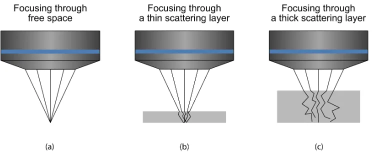
Figure 1.9: Scattering regimes. (a) In free space, conventional lenses form the correct wavefronts to focus light to tight focal spots. (b) When the scattering medium is thin and the thickness is less than the mean free path (L < l), most of the light is unscattered and conventional lenses can still form relatively tight focal spots. (c) Once the thickness exceeds the transport mean free path (L > l∗), conventional lenses can no longer form effective focal spots since almost all the light has been multiply scattered and very little ballistic light remains.

refracts. These processes more generally are referred to as elastic scattering, because the wavelength of light is not changed due to the scattering interaction. This is in contrast to other inelastic scattering process such as Raman or Brillouin scattering where the scattered photons are of different energies than the incoming photons.

(37)

Time-reversal symmetry of the wave equation

Although the heterogeneous refractive index distributions in scattering media present a challenge for focusing light through them, the physics of the wave equation can help to simplify the situation. Among the most important properties of the wave equation for sending light through scattering media is the time-reversal symmetry of the wave equation. In the linear regime, the electric fieldE(r,t)of an electromagnetic wave can be described by the wave equation

µ(r)(r)∂ 2E

∂t2 = ∇ 2E,

(1.27)

where and µare the position dependent electric and magnetic permeabilities of the medium, respectively. Recalling that the refractive index is defined asn=

√

rµr

wherer = ₀ and µr =

µ

µ₀ are the relative electric and magnetic permeabilities, this gives a wave equation in terms of the local refractive index as

n(r)2

c2 0

∂2E

∂t2 = ∇ 2E,

(1.28)

wherec0is the speed of light in vacuum.

The time-reversal symmetry property means that ifE(r,t)is a solution to the wave equation, thenE(r,−t)is also a valid solution. For example, ifE(r,t)is a spherical wave emanating from a source, then E(r,−t)is a spherical wave converging back toward the source. In the context of scattering media, this means that the time-reversed copy of a scattered light field will reverse its course through the scattering medium and converge at its original source. The benefits of using time-reversal to send waves through scattering media was first discovered and developed by Matthias Fink and colleagues using ultrasonic waves in the late 1980s. Interested readers are directed to reference [8] for more detailed information.

Transmission Matrix

(38)

[image:38.612.215.395.76.308.2]

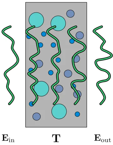
Figure 1.10: A an example of the transmission matrix terminology for

wave-fronts passing through scattering media. The input fieldEin passes through the

transmission matrixTwhich maps it onto the output fieldEout.

and output mode. While the concept of the transmission matrix is a general one in engineering, it has only been in the past decade that this concept has been explored in optics due to the growing availability of tools such as highly sensitive and fast cameras, which enable precise measurement of many optical modes, and spatial light modulators (SLMs), which enable the manipulation of many individual optical modes. Figure 1.10 and Equation 1.30 show a schematic and mathematical description of how the transmission matrix is defined.

E_out=T E_in (1.29)

         

E_out₁

E_out₂

...

E_out_m

          =          

t₁₁ t₁₂ . . . t₁n

t₂₁ t₁₂ . . . t₂n

... ... ... ...

tm1 tm2 . . . tmn

                   

E_in₁

E_in₂

...

E_in_n

          (1.30)

(39)

field pattern. Furthermore, the fact that wave propagation is time-symmetric means that time-reversal can be used to find the appropriate input light patterns. As demonstrated in reference [9] by Popoff and colleagues, one can use the time-reversal operator to find the correct input fieldEinto use in order to obtain a desired

output fieldEtarget. In the case where the input light is monochromatic, time-reversal

is the same a phase conjugation. Therefore, the optimized pattern to generate an output target fieldEtarget, is given by

E_in =T†E_target, (1.31)

where the†indicates conjugate transpose.

When inputting this input field, the resulting output is given by

E_out =O_focE_in (1.32)

where the operatorOfoc =T

†

T is called the time-reversal operator.

To further analyze the properties of this matrix, we can perform a singular value decomposition of the matrix. This will decompose the m×ntime-reversal matrix O_focinto the form

O_foc =UΣV∗, (1.33)

whereU is an m×m complex unitary matrix whose columns are the left singular vectors, Σ is an m× n with non-negative real numbers on the diagonal, andV is ann×ncomplex unitary matrix whose columns are the right singular vectors. In the context of the transmission matrix, theU acts to map the input modes onto the eigenmodes of the system,Σcontains the eigenvalues of the time-reversal operator matrix, andV acts to map the eigenmodes onto the output modes.

(40)

situations such as scattering in biological tissue, although absorption is low, the total energy is not conserved due to the limited collection efficiency. This causes the transmission matrix elements to become uncorrelated and follow a random, complex Gaussian distribution and, as follows from random matrix theory, the singular value distribution obeys a Marchenko-Pastur or quarter-circle distribution where nearly all the open channels have disappeared. Further details and additional papers for those interested are discussed in reference [9].

1.5 Wavefront shaping

However, even though the open channels begin to disappear, the presence of partially open channels means that we can still control the light propagation through the scattering medium. Since the transmission matrix is a linear amplitude and phase mapping between input modes and output modes, the output field at a particular point can be enhanced.

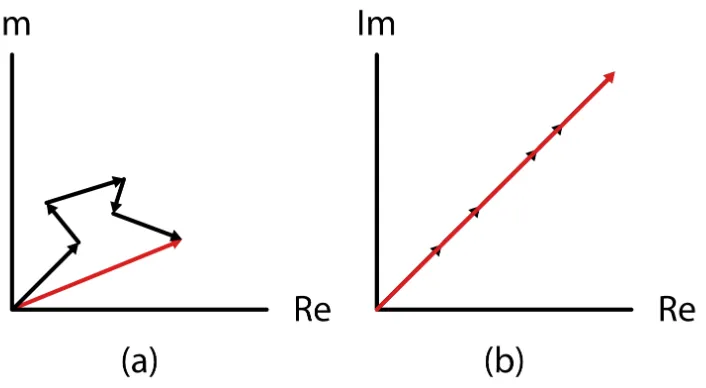
Wavefront shaping in optics was first demonstrated in 2007 by Vellekoop and Mosk [10]. In essence, the goal of creating a focus is to create a point of constructive in-terference through the scattering media and cause the contributions from individual output modes to align in phase. When we send coherent light through a scattering medium, the resulting output light field manifests as a "speckle" pattern. This is due to the random nature of the transmission matrix and is due to the random interference of the contributions from different output modes. At a given output mode, we can visualize the situation as a phasor diagram, where each individual phasor represents the amplitude and phase contribution at the selected output mode from a collection of input modes.

(41)

[image:41.612.136.489.80.274.2]

Figure 1.11: Phasor diagram illustrating the interference of different modes in

a speckle pattern. (a) If the phasors are not aligned, they follow a 2D random walk in the complex plane. The red vector indicates the resultant phasor sum. (b) If the phasors are controlled via wavefront shaping, the phasors can be rotated so that they are in phase with one another to form a constructive interference peak. This creates an enhancement in the intensity at the point of interest given by the increase in the length of the resultant vector in (b) compared to (a).

plane.

Another point of practical benefit is that this control doesn’t require full control of both the amplitude and phase of the input field. While amplitude control would enable us to change the length of the vectors, we can see that control over the phase alone (allowing us to rotate the vectors in the complex plane) is enough to enable an enhancement at the output mode of interest. To do this, we simply adjust the phase of the phasors, thereby rotating them to maximize the length of the resultant vector. This is useful because it is much easier in practice to control either the phase or amplitude only of an input field with a spatial light modulator instead of simultaneously controlling both.

Wavefront shaping in practice

(42)

displayed. There are a variety of different feedback-based methods that have been developed and are nicely described in a recent review, reference [12].

The main drawback of feedback-based wavefront shaping methods is that they are slow because many measurements need to be made. This problem is solved by the time-reversal-based methods. With time-reversal, we use a source of coherent light emanating from a point of interest through or inside the scattering medium and measure the scattered wavefront corresponding to this source. Then, by creating the time-reversed or phase-conjugated version of that scattered wavefront, light can be focused back on the original point source. The advantage of this method is that it can achieve fast focusing speeds, since it requires only a single measurement of the scattered field in comparison to feedback-based methods, which require many mea-surements to form a high fidelity focus. However, this method requires a much more complicated optical setup to perform the time-reversal. This was originally demon-strated with an analog time-reversal mirror based on a photorefractive crystal [13] but now is commonly accomplished using a digital time-reversal mirror composed of a camera and spatial light modulator [14]. While this digital implementation increases the flexibility of the system and enables more energy to be played back in the time-reversed wavefront compared to the analog systems, it requires precise, pixel-to-pixel alignment of the camera and spatial light modulator which makes the system challenging to build, even with the development of algorithms to help with the alignment procedure [15].

Wavefront shaping with guidestars

Up until now, we have discussed how wavefront shaping can help to focus light through scattering medium, but for practical applications, we want to focus light inside scattering media like biological tissue. To do this, we need an additional

component in our wavefront shaping system called a guidestar. Borrowed from concepts in astronomy where stars serve as effective point sources outside the atmosphere to help find the correct wavefront solution for the deformable mirrors on the earth’s surface to correct for the aberration of the atmosphere, guidestars in the context of wavefront shaping provide information about the correct wavefront solution to focus at a point inside the tissue.

(43)

[image:43.612.118.497.67.213.2]

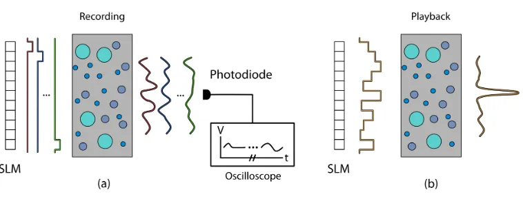
Figure 1.12: Feedback-based wavefront shaping. Feedback-based wavefront shap-ing uses a signal from a desired focal location as a feedback signal and creates different, orthogonal input patterns to maximize the intensity at that location. (a) In a basic scheme, a photodiode can be used to measure the light intensity at a given output point as different input patterns are displayed on a spatial light modulator (SLM). (b) After measuring several patterns, a best pattern can be composed to enhance the light at the desired location.

kinetic, and ultrasound-based guidestars. Light-based guidestars include approaches using fluorescence, second-harmonic generation, and absorption. These techniques are generally simple, but suffer from low efficiency and are often incompatible with time-reversal methods, since they generally do not generate coherent light.

(44)

[image:44.612.119.499.75.284.2]

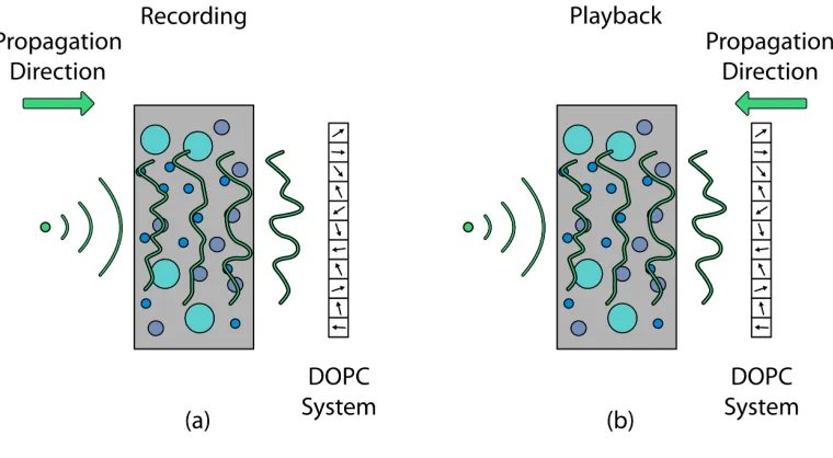
Figure 1.13: Time-reversal-based wavefront shaping. Time-reversal-based wave-front shaping uses the scattered light from a source of light within the sample and then sends a time-reversed copy of that wavefront back into the scattering medium to focus back on the location of the original source. The operation is broken down into two stages (a) recording and (b) playback. (a) In the recording stage, the scattered wavefront from a guidestar or location of interest is measured. (b) In the playback stage, the time-reversed copy of the wavefront is generated and displayed on the spatial light modulator (SLM). This time-reversed copy scatters back through the medium and constructively interferes to form a focus at the location of the original light source.

the downside of these methods is that they require the physical implantation of an external particle or rely on moving objects like red blood cells in the tissue to create a focus that reduces the control over the focusing location.

(45)

1.6 Decorrelation

The preceding description of the transmission matrix and wavefront shaping assumes that the system is stable in time and that the matrix elements are fixed. However, if the configuration of the scattering medium changes (e.g., particles in a suspension move due to convection or Brownian motion, blood flows through a tissue sample, or a sample moves due to mechanical instability), the elements of the transmission matrix will also change. We call this process decorrelation since the transmission matrix elements lose correlation over time. In practice, when we want to focus light through or inside a scattering medium, we rely on the time-symmetry of the medium and stability of the transmission matrix to do so. Movement breaks the time-symmetry of the wave equation. This means that the time-reversed wavefront solution that would normally create a strong focus at the location of interest is no longer valid.

For practical applications, the speed at which this decorrelation takes place is very important, since it sets the boundaries of what practical applications can be addressed with wavefront shaping. Therefore, knowing this decorrelation speed for a particular type of medium is important.

1.7 Outline of this thesis

The remainder of this thesis is structured as follows. Chapter 2 investigates the decorrelation procedure in acute rat brain slices and its relationship to the tissue thickness in the absence of blood flow. Chapter 3 extends this investigation to the mouse brainin-vivo and compares the decorrelation times with those found in the absence of blood. This helps to establish bounds for the practical applications of wavefront shaping technologies and also provides guidance for future technology development.

Next, we explore the practical application of time-reversed ultrasonically-encoded (TRUE) light focusing in brain tissue to improve light delivery for optogenetics in Chapter 4.

(46)

References

[1] H. C. Hulst,Light scattering by small particles. Courier Corporation, 1981.

[2] J. W. Goodman,Statistical optics. John Wiley & Sons, 2015.

[3] D. Huang, E. A. Swanson, C. P. Lin, J. S. Schuman, W. G. Stinson, W. Chang, M. R. Hee, T. Flotte, K. Gregory, C. A. Puliafito, et al., “Optical coherence tomography,”science, vol. 254, no. 5035, pp. 1178–1181, 1991.

[4] D. Gabor, “A new microscopic principle,” Nature, vol. 161, pp. 777–778, 1948.

[5] E. N. Leith and J. Upatnieks, “Reconstructed wavefronts and communication theory,”JOSA, vol. 52, no. 10, pp. 1123–1130, 1962.

[6] N. Verrier and M. Atlan, “Off-axis digital hologram reconstruction: Some practical considerations,”Applied Optics, vol. 50, no. 34, H136–H146, 2011.

[7] L. V. Wang and H.-i. Wu, Biomedical optics: principles and imaging. John Wiley & Sons, 2012.

[8] M. Fink, “Time reversal of ultrasonic fields. i. basic principles,”IEEE trans-actions on ultrasonics, ferroelectrics, and frequency control, vol. 39, no. 5, pp. 555–566, 1992.

[9] S. Popoff, G. Lerosey, R. Carminati, M. Fink, A. Boccara, and S. Gigan, “Measuring the transmission matrix in optics: An approach to the study and control of light propagation in disordered media,” Physical Review Letters, vol. 104, no. 10, p. 100 601, 2010.

[10] I. M. Vellekoop and A. Mosk, “Focusing coherent light through opaque strongly scattering media,” Optics Letters, vol. 32, no. 16, pp. 2309–2311, 2007.

[11] J. W. Goodman, Speckle phenomena in optics: theory and applications. Roberts and Company Publishers, 2007.

[12] I. M. Vellekoop, “Feedback-based wavefront shaping,”Optics Express, vol. 23, no. 9, pp. 12 189–12 206, 2015.

[13] Z. Yaqoob, D. Psaltis, M. S. Feld, and C. Yang, “Optical phase conjugation for turbidity suppression in biological samples,” Nature Photonics, vol. 2, no. 2, p. 110, 2008.

[14] M. Cui and C. Yang, “Implementation of a digital optical phase conjugation system and its application to study the robustness of turbidity suppression by phase conjugation,”Optics Express, vol. 18, no. 4, pp. 3444–3455, 2010.

(47)

[16] E. H. Zhou, H. Ruan, C. Yang, and B. Judkewitz, “Focusing on moving targets through scattering samples,”Optica, vol. 1, no. 4, pp. 227–232, 2014.

[17] C. Ma, X. Xu, Y. Liu, and L. V. Wang, “Time-reversed adapted-perturbation (TRAP) optical focusing onto dynamic objects inside scattering media,” Na-ture Photonics, vol. 8, no. 12, p. 931, 2014.

[18] H. Ruan, T. Haber, Y. Liu, J. Brake, J. Kim, J. M. Berlin, and C. Yang, “Fo-cusing light inside scattering media with magnetic-particle-guided wavefront shaping,”Optica, vol. 4, no. 11, pp. 1337–1343, 2017.

(48)

C h a p t e r 2

THE RELATIONSHIP BETWEEN DECORRELATION AND

TISSUE THICKNESS IN ACUTE RAT BRAIN TISSUE SLICES

This chapter is adapted from the manuscript J. Brake†, M. Jang†, and C. Yang, “Analyzing the relationship between decorrelation time and tissue thickness in acute rat brain slices using multispeckle diffusing wave spectroscopy,” JOSA A, 33(2), pp. 270–275, 2016.

2.1 Abstract

Novel techniques in the field of wavefront shaping have enabled light to be focused deep inside or through scattering media such as biological tissue. However, most of these demonstrations have been limited to thin, static samples since these tech-niques are very sensitive to changes in the arrangment of the scatterers within. As the samples of interest get thicker, the influence of the dynamic nature of the sample becomes even more pronounced and the window of time in which the wavefront solutions remain valid shrinks further. In this chapter, we examine the time scales upon which this decorrelation happens in acute rat brain slices via multispeckle dif-fusing wave spectroscopy and investigate the relationship between this decorrelation time and the thickness of the sample using diffusing wave spectroscopy theory and Monte Carlo photon transport simulation.

2.2 Wavefront shaping and decorrelation time

The optical opacity of biological tissue in the visible regime has long been a challenge in the field of biomedical optics. Since the light traveling through thick samples undergoes many scattering events, the information about the sample is scrambled and the light field exiting the sample forms a random speckle pattern [1].

(49)

unscattered or singly-scattered portion of light passing through the sample, these wavefront shaping techniques incorporate even multiply scattered portions of the scattered light field.

While these wavefront shaping techniques have been primarily demonstrated with static scattering samples or fixed biological tissues, the ability to apply these tech-niques to living biological tissues is the ultimate goal. The main challenge facing this development is the dynamic nature of living tissue. In biological tissue where the average number of scattering events for an individual photon traveling through the sample is very large, small changes in the composition of the sample can break the time-reversal symmetry of optical scattering and cause a mismatch between the shaped wavefront and the correct wavefront solution, severely degrading the qual-ity of the shaped focus. From previous studies, it is known that this degradation is proportional to the intensity autocorrelation function of the scattered light - a conventional measure of scatterer movement [7].

In this study, we measure the intensity autocorrelation function of acute brain tissue slices from rats and examine the relationship between the characteristic decorrelation time and tissue thickness, comparing the results with the theoretical predictions of diffusing wave spectroscopy (DWS), which suggest that the decorrelation time should be inversely proportional to the square of the thickness [8–12]. The results of this study elucidate the timescale on which the movement inside tissue occurs and guide the further development of fast wavefront shaping techniques, especially toward the development of improved light delivery techniques for optogenetics both onin vitroacute brain slices and eventually forin vivoapplications [13–16].

2.3 Multispeckle diffusing wave spectroscopy

(50)

(DWS) [8, 10, 17].

The main aim of DWS is to relate the decorrelation of the scattering media due to the movement of the scatterers to the decay of the autocorrelation of the measured electric field. As derived by Maret and Wolf [17], the electric field autocorrelation in the case of multiple scattering and Brownian motion particle diffusion can be written as

g₁(τ)=

∫ ∞

0

P(s)_exp −2τ

τ₀

s l∗

ds, (2.1)

where τ is delay time, τ0 = 1/

Dk2 0

is the characteristic decay time, k0 = 2π/λ

is the wavenumber of the light in the medium, D is the diffusion constant of the scattering particles, l∗ is the transport mean free path, s is the path length, and P(s)_{is the distribution of path lengths in the medium. From this equation, we can}

see that the field autocorrelation is essentially a weighted sum (weights P(s)) of exponential decays at rates set byD, k0,l

∗

, ands. However, by examining different thicknesses of the same sample in the same experimental configuration, D, k0, and

l∗ are essentially fixed. Therefore, we can directly probe the relationship between

the thickness and the characteristic decay time by determining the dependence of P(s)_{on the thickness.}