SEG SSC: a framework based on synthetic examples generation for self labeled semi supervised classification

(1)

SEG-SSC: A Framework based on Synthetic

Examples Generation for Self-Labeled

Semi-Supervised Classification

Isaac Triguero, Salvador Garc´ıa, and Francisco Herrera

Abstract—Self-labeled techniques are semi-supervised classifi-cation methods that address the shortage of labeled examples via a self-learning process based on supervised models. They progressively classify unlabeled data and use them to modify the hypothesis learned from labeled samples. Most relevant proposals are currently inspired by boosting schemes to iteratively enlarge the labeled set. Despite their effectiveness, these methods are constrained by the number of labeled examples and their distri-bution, which in many cases is sparse and scattered. The aim of this work is to design a framework, named SEG-SSC, to improve the classification performance of any given self-labeled method by using synthetic labeled data. These are generated via an oversampling technique and a positioning adjustment model that use both labeled and unlabeled examples as reference. Next, these examples are incorporated in the main stages of the self-labeling process. The principal aspects of the proposed framework are: (a) introducing diversity to the multiple classifiers used by using more (new) labeled data, (b) fulfilling labeled data distribution with the aid of unlabeled data, and (c) being applicable to any kind of self-labeled method. In our empirical studies, we have applied this scheme to four recent self-labeled methods, testing their capabilities with a large number of data sets. We show that this framework significantly improves the classification capabilities of self-labeled techniques.

Index Terms—Self-Labeled methods, co-training, synthetic ex-amples, semi-supervised classification.

I. INTRODUCTION

H

AVING a multitude of unlabeled data and few labeled ones occurs quite often in many practical applications such as medical diagnosis, spam filtering, bioinformatics, etc. In this scenario, learning appropriate hypotheses with tradi-tional supervised classification methods [1] is not straightfor-ward because they only can exploit labeled data. Nevertheless, Semi-Supervised Classification (SSC) [2], [3], [4] approaches also utilize unlabeled data to improve the predictive per-formance, modifying the learned hypothesis obtained from labeled examples alone.

With SSC we may pursue two different objectives: trans-ductive and intrans-ductive classification [5]. The former is devoted to predicting the correct labels of a set of unlabeled examples that is also used during the training phase. The latter refers

This work was supported by the Research Projects TIN2011-28488, P10-TIC-6858 and P11-TIC-7765.

I. Triguero and F. Herrera are with the Department of Computer Science and Artificial Intelligence of the University of Granada, CITIC-UGR, Granada, Spain, 18071. E-mails:{triguero, herrera}@decsai.ugr.es

Salvador Garc´ıa is with the Department of Computer Science of the University of Ja´en Ja´en, Spain, 23071. E-mail: [email protected]

to the problem of predicting unseen data by learning from labeled and unlabeled data as training examples. In this work, we will analyze both settings.

Existing SSC algorithms are usually classified depending on the conjectures they make about the relation of labeled and unlabeled data distributions. Broadly speaking, they are based on the manifold and/or cluster assumption. The man-ifold assumption is satisfied if data lie approximately on a manifold of lower dimensionality than the input space [6]. The cluster assumption states that similar examples should have the same label. Graph-based models [7] are the most common approaches to implementing the manifold assumption [8]. As regards examples of models based on the cluster assumption, we can find generative models [9] or semi-supervised support vector machines [10]. Recent studies have addressed multiple assumptions in one model [11], [5], [12].

Self-labeled techniques are SSC methods that do not make any specific suppositions about the input data [13]. These models use unlabeled data within a supervised framework via a self-training process. First attempts correspond to the self-training algorithm [14] that iteratively enlarges the la-beled training set by adding the most confident predictions of the supervised classifier used. The standard co-training [15] methodology splits the feature space into two different conditionally independent views. Then, it trains one classifier in each specific view, and the classifiers teach each other the most confidently predicted examples. Advanced approaches do not require explicit feature splits or the iterative mutual-teaching procedure imposed by co-training, as they are com-monly based on disagreement-based classifiers [16], [17], [18]. These models have been successfully applied to many real applications such as image classification [19], shadow detection [20], computer-aided diagnosis [21], etc.

Self-labeled techniques are limited by the number of labeled points and their distribution to identifying reliable unlabeled examples. This problem is more pronounced when the labeled ratio is greatly reduced and labeled examples do not minimally represent the domain. Moreover, most of the advanced models use some diversity mechanisms, such as bootstrapping [22], to provide differences between the hypotheses learned with the multiple classifiers. However, these mechanisms may provide a similar performance to classical self-training or co-training approaches if the number of labeled data is insufficient to achieve different learned hypotheses.

(2)

to multiple classifier approaches and fulfill the labeled data distribution. A complete motivation for the use of synthetic labeled examples is discussed in Section III-A.

We propose a framework applicable to any self-labeled method that incorporates synthetic examples in the self-learning process. We will denote this framework “Synthetic Examples Generation for Self-labeled Semi-supervised Clas-sification” (SEG-SSC). It is composed of two main parts: generation and incorporation.

• The generation process consists of an oversampling tech-nique and a later adjustment of the positioning of the examples. It is initially inspired by the SMOTE algorithm [23] to generate new synthetic examples, for all the classes, based on both the small labeled set and the unlabeled data. Then, this process is refined using a positioning adjustment of prototypes model [24] based on a differential evolution algorithm [25].

• New labeled points are then included in two of the main steps of a self-labeling method: the initialization phase and the update of the labeled training set, so that it introduces new examples in a progressive manner during the self-labeling process.

An extensive experimental analysis is carried out to check the performance of the proposed framework. We apply the SEG-SSC scheme to four recent self-labeled techniques that have different characteristics, comparing the performance ob-tained with the original proposals. We conduct experiments over 55 standard classification data sets extracted from the KEEL and UCI repositories [26], [27] and 11 high dimensional data sets from the book by Chapelle et al. [2]. The results will be contrasted with nonparametric statistical tests [28], [29].

The remainder of this paper is organized as follows. Section II defines the SSC problem and sums up the classical and current self-labeled approaches. Then, Section III presents the proposed framework, explaining its motivation and the details of its implementation. Section IV describes the experimental setup and discusses the results obtained. Finally, Section V summarizes the conclusions drawn in this work.

II. SELF-LABELEDSEMI-SUPERVISEDCLASSIFICATION

This section provides the definition of the SSC problem (Section II-A) and briefly describes the most relevant self-labeled approaches proposed in the literature (Section II-B).

A. Semi-supervised classification

A formal description of the SSC problem is as follows: Let

xp be an example wherexp = (xp1,xp2, ...,xpD, ω), with xp belonging to a class ω and a D-dimensional space in which

xpi is the value of thei-th feature of the p-th sample. Then, let us assume that there is a labeled set L which consists of

n instances xp withω known and an unlabeled setU which consists of m instancesxq with ω unknown, let m > n. The

L∪U set forms the training setT R. Moreover, there is a test set T S composed oft unseen instancesxr withω unknown, which has not been used at the training stage.

The aim of SSC is to obtain a robust learned hypothesis usingT Rinstead ofLalone. It can be applied in two slightly

different settings. On the one hand, transductive learning is de-voted to classify all theminstancesxq ofU with their correct class. The class assignation should represent the distribution of the classes efficiently, based on the input distribution of

L and U. On the other hand, the inductive learning phase consists of correctly classifying the instances ofT S based on the previously learned hypothesis.

B. Self-labeled techniques: previous work

Self-labeled techniques form an important family of meth-ods in SSC [3]. They are not intrinsically geared to learning in the presence of both labeled and unlabeled data, but they use unlabeled points within a supervised learning paradigm. These techniques aim to obtain one (or several) enlarged labeled set/s, based on the most reliable predictions. Thus, these models do not make any specific assumptions about the input data, but the models accept that their own predictions tend to be correct. Some authors state that self-labeling is likely to be the case when the classes form well-separated clusters [3] (cluster assumption).

The major benefits of this family of methods are: simplicity and being a wrapper methodology. The former is related to the facility of implementation and applicability. The latter means that any kind of classifier can be used regardless of its complexity, which is very important depending on the problem tackled. As caveats, the addition of wrongly labeled examples during the self-labeling process can lead to an even worse performance. Several mechanisms have been proposed to reduce this problem [30].

A preeminent work with this philosophy is the self-training paradigm designed by Yarowsky [14]. In self-training, a su-pervised classifier is initially trained with theLset. Then it is retrained with its own most confident predictions, enlarging its labeled training set. Thus, it is defined as a wrapper method for SSC. This idea was later extended by Blum and Mitchell [15] with the method known as co-training. This consists of two classifiers that are trained on two sufficient and redundant sets of attributes. This requirement implies that each subset of features should be able to perfectly define the frontiers between classes. Then, the method follows a mutual teaching procedure that works as follows: each classifier labels the most confidently predicted examples from its point of view and they are added to theLset of the other classifier. It is also known that usefulness is constrained by the imposed requirement [31], which is not satisfied in many real applications. Nevertheless, this method has become an example for recent models thanks to the idea of using the agreement (or disagreement) of multiple classifiers and the mutual teaching approach. A good study of when co-training works can be found in [32].

(3)

alternative, named Democractic co-learning (Democratic-Co) [34], which is also based on multi-learning. As an alternative, which requires neither sufficient and redundant views nor several supervised learning algorithms, Zhou and Li [35] pre-sented the Tri-Training algorithm, which attempts to determine the most reliable unlabeled data as the agreement of three clas-sifiers (same learning algorithm). Then, they proposed the Co-Forest algorithm [21] as a similar approach that uses Random Forest [36]. A further similar approach is Co-Bagging [37], [38] where confidence is estimated from the local accuracy of committee members. Other recent self-labeled approaches are [39], [40], [41], [42], [43].

In summary, all of these recent schemes work on the hypothesis that several weak classifiers, learned with a small number of instances, can produce better generalizations than only one weak classifier. These methods are also known as disagreement-based models that are motivated, in part, by the empirical success of ensemble learning. The term disagreement-based was recently coined by Zhou and Li [17].

III. SYNTHETIC EXAMPLES GENERATION FOR

SELF-LABELED METHODS.

In this section we present the SEG-SSC framework. Firstly, Section III-A enumerates the arguments that justify our pro-posal. Secondly, Section III-B explains how to generate useful synthetic examples in a semi-supervised scenario. Finally, Section III-C describes the SEG-SSC framework, emphasizing when synthetic data should be used.

A. Motivation: Why add synthetic examples?

The most important weakness of self-labeling models can occur when erroneous labeled examples are added to the labeled training set. This will incorrectly modify the learned model, which may lead to the addition of wrong examples in successive iterations. Why does this situation occur?

• There may be outliers in the original unlabeled set. This problem can be avoided if they are detected and not included in the labeled training set. For this problem, there are several solutions in the literature such as edition schemes [30], [44], [45] or some other mechanisms [33]. Recent models, such as Tri-Training [35] or Co-Forest [21], establish some criteria to compensate for the negative influence of noise by augmenting the labeled training set with sufficient new labeled data.

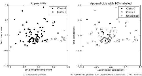
• Independently of the number of unlabeled examples, they can be limited by the distribution of labeled input data. If the available labeled instances do not represent a reliable domain of the problem, it may complicate the estimation of confidence predictions because the super-vised classifiers used do not have enough information to establish coherent hypotheses. Furthermore, it is even more difficult if these labeled points are very close to the decision boundaries. Figure 1 shows an example with the appendicitis problem [27]. This picture presents a two-dimensional projection (obtained with PCA [46]) of the problem and a partition with 10 % of labeled examples. As we can observe, not only is the problem not well

represented by labeled points, it also shows that some of the nearest unlabeled points to the two labeled examples of class 1 (blue circles) belong to class 0 (red crosses). This fact can affect confidence of a self-labeled method estimated with the base classifier.

• A greatly reduced labeled ratio may produce a lack of diversity among self-labeling methods with more than one classifier. As we have established above, multiple classifier approaches work as a combination of several weak classifiers. However, if there are only a few labeled data it is very difficult to obtain different hypotheses, and therefore, the classifiers are identical. For example, the Tri-Training algorithm is based on a bootstrapping approach [22]. This re-sampling technique creates new labeled sets for each classifier by modifying the original

L. In general, this operation yields different labeled sets to the original, but it is not significant in the case of small labeled data sets and the existence of outliers in the sample. As a consequence, it could lead to biased ex-amples which will not accurately represent the domain of the problem. Although multi-learning approaches attempt to achieve diversity by using different kinds of learning models, a reduced number of instances usually damages their performance because the models are too weak. The first limitation has already been addressed in the literature with different mechanisms [47]. However, the last two issues are currently open problems.

In order to ease both situations, mainly induced by the shortage of labeled points, we introduce new labeled data into the self-labeling process. To do this, we rely on the success of oversampling approaches in imbalanced domains [48], [49], [50], [51], but with the difference that we deal with all the classes of the problem.

Nevertheless, the use of synthetic data for self-labeling methods is not straightforward and must be carefully per-formed. The aim of using an oversampling method is to effectively reinforce the decision regions between classes. To do so, we will be aided by the distribution of unlabeled data in conjunction with the labeled ones, because if we focus only on labeled examples, it may lead to generate noisy instances when the second issue explained above happens. The effectiveness of this idea will be empirically checked in Section IV.

B. Generation of synthetic examples

(4)

−1.0

−0.5

_{1st principal component}

0.0

0.5

1.0 −1.0

−0.5

0.0

0.5

1.0 2n

d c

om

po

ne

nt

Appendicitis

Class 0

Class 1

(a) Appendicitis problem

−1.0

−0.5

0.0

0.5

1.0 1st principal component

−1.0

−0.5

0.0

0.5

1.0 2n

d c

om

po

ne

nt

Appendicitis with 10% labeled

Class 0

Class 1

Unlabeled

[image:4.612.57.558.59.328.2]

(b) Appendicitis problem: 10% Labeled points (Democratic - 0.7590 accuracy.)

Fig. 1. Two-dimensional projections of Appendicitis. Red circles, class 0. Blue squares, class 1. White triangles, unlabeled.

1: Input:Labeled setL, Unlabeled setU, Oversampling factorf, Number of Neighborsk.

2: Output:OverSampledset. 3: OverSampled=∅ 4: T R=L∪U

5: ratio=f·#T R #L

6: RandomizeT R

7: fori= 1toN umberOf Classesdo

8: P erClass[i]= getFromClass (L,i) 9: forj= 1to#P erClass[i]do

10: Generated= 0 11: repeat

12: neighbors[1..k]= Computeknearest neighbors forP erClass[i][j]inT R

13: nn= Random number between 1 andk

14: Sample=P erClass[j] 15: N earest=T R[neighbors[nn]] 16: form= 1toN umberOf Attributesdo

17: dif=N earest[m]−Sample[m]

18: gap= Random number between 0 and 1.

19: Synthetic[m] =Sample[m] +gap∗dif

20: end for

21: OverSampled=OverSampled∪Synthetic

22: Generated+ + 23: untilGenerated < ratio

24: end for

25: end for

26: OverSampled=DE adjustment(OverSampled,L) 27: return OverSampled

Algorithm 1:Generation of synthetic examples

Initialization: We start from theLandU sets as well as an user-defined oversampling factorf and a numberkof nearest neighbors. We will generate a set of synthetic prototypes

OverSampledthat is initialized as empty (Instruction 3).

The ratio of synthetic examples to be generated is computed according tof and the proportion of labeled examples in the

training set T R (See instructions 4 and 5). Furthermore, to prevent the influence of the order of labeled and unlabeled instances when computing distances, theT Rset is randomized (Instruction 6).

Next, the algorithm enters a loop (Instructions 7-25) to proportionally oversample each class, using its own labeled samples as the base. Thus, we extract fromL a set of

exam-ples P erClass that belong to the current class (Instruction

8). Each one will serve as the base prototype and will be oversampled as many times as the previous computed ratio indicates (Instructions 11-23).

New synthetic examples are located along the line segments joining any of theknearest neighbors (randomly chosen). To face the SSC scenario, the nearest neighbors are not only being looked for in the L set, but are searched for in the T R set (Instruction 12). In this way, we try to avoid the negative effects of the second weakness of self-labeled techniques explained before. Following the idea of SMOTE, synthetic examples are initially generated as the difference between an existing sample and one of its nearest neighbors (Instruction 17). Then, this difference is scaled by a random number in the range [0,1], and is added to the base example (Instruction 18 and 19). It is noteworthy that the class value of the generated example is the same as the considered base sample. The generated prototypes are iteratively stored in OverSampled

until the stopping condition is satisfied.

(5)

self-labeling approaches and their confidence predictions. It is well-known that SMOTE can generate noisy data [53] which are usually eliminated with edition schemes. Because we are not interested in removing synthetic data, we will apply an evolutionary adjustment process to the OverSampled set (Instruction 26) based on the differential evolution algorithm used in [54].

Differential evolution [25] follows the general procedure of an evolutionary algorithm [55]. It starts with a set of candidate solutions, the so-called individuals, which evolve during a determined number of generations through differ-ent operators: mutation, crossover and selection; aiming to minimize/maximize a fitness function. For our purposes, this algorithm is adapted in the following way:

• Each individual encodes a single prototype. The process consists of the optimization of the location of all the individuals of the population.

• Mutation and crossover operators guide the optimization of the positioning of the prototypes. These operators only produce modifications to the attributes of the prototypes of the OverSampled set, keeping the class value un-changeable throughout the evolutionary cycle. We will focus on the DE/CurrentToRand/1 strategy to generate new prototypes [56].

• Then, we obtain a new set of synthetic prototypes that should be evaluated to decide whether it is better or not than the current set. To make this decision, we use the most reliable data we have, that is, the labeled data L. The generated data should be able to correctly classify

L. To check this, the nearest neighbor rule is used as the base classifier to obtain the corresponding fitness value. We try to maximize this value.

The stopping criteria is achieved when the generated data perfectly classifyL, or a given number of iterations have been performed. More details in Section III.B of reference [54].

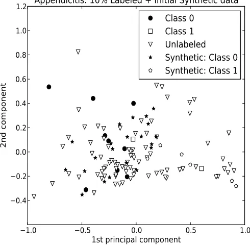
It is worth mentioning that this optimization process is only applied to cases in which the former oversampling approach generates synthetic data that is not able to classify

L. We thereby endow our model with greater robustness. Figure 2 shows an example of a resulting set of over-sampled prototypes in the appendicitis problem. We can observe that in comparison with Figure 1, the available labeled data points better represent the domain of the problem.

C. Self-labeling with synthetic data

In this subsection, we describe the SEG-SSC framework in depth. With the generation method presented, we obtain new labeled data that can be directly used to improve the generalization capabilities of self-labeled approaches. Never-theless, the aim of this framework is to be as flexible as possible, so that it can be applied to different self-labeled algorithms. Although each method proceeds in a different way, they either share some operations or are very similar. Therefore, we explain how to incorporate synthetic examples in the self-learning process in order to address the limitations on the distribution of labeled data and the lack of diversity in multiple classifier methods.

−1.0 −0.5 0.0 0.5 1.0

1st

principal componen

−0.4

−0.2

0.0

0.2

0.4

0.6

0.8

1.0

1.2 2n

d

co

m

po

ne

n

Appendici is: 10% Labeled + Ini ial Syn he ic da a

Class 0

[image:5.612.316.561.61.303.2]

Class 1

Unlabeled

Syn he ic: Class 0

Syn he ic: Class 1

Fig. 2. Example of data generation in the Appendicitis problem. Two-dimensional projections of Appendicitis. Red circles, class 0. Blue squares, class 1. White triangles, unlabeled. Red stars, synthetic class 0. Blue pen-tagons, synthetic class 1. (SEG-SSC+Democratic - 0.8072 accuracy.)

In general, self-labeled methods use a set of N classifiers

Ci, wherei ǫ[1, N], to predict the class of unlabeled instances. Each Ci has an associated labeled set Li that is iteratively enlarged. In what follows, we describe the three main opera-tions that support our proposal. For clarity, Figure 3 depicts a flowchart of the proposed scheme, outlining its more general operations and way of working.

• Initialization of classifiers: In current approaches,Li is initially formed from the available data inL. Depending on the particular method, they may use the same labeled data for each Li or apply a bootstrapping to introduce diversity. As we showed before, both alternatives can lead to a lack of diversity when more than one classifier is used. To solve this, we promote the generation of different synthetic examples for each classifierCi. In this way, the generation mechanism is applied a total of N

times. Because L data are the most confident examples, we ensure that they belong to eachLiin conjunction with synthetic examples. Note that the generation method has some randomness, so different executions generate dis-tinct synthetic points. This ensures the diversity between

Li sets.

(6)

[image:6.612.51.301.425.468.2]

Fig. 3. SEG-SSC flowchart

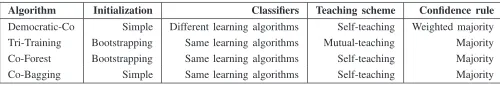
TABLE I

MAIN CHARACTERISTICS OF SELECTED SELF-LABELED METHODS

Algorithm Initialization Classifiers Teaching scheme Confidence rule Democratic-Co Simple Different learning algorithms Self-teaching Weighted majority Tri-Training Bootstrapping Same learning algorithms Mutual-teaching Majority Co-Forest Bootstrapping Same learning algorithms Self-teaching Majority Co-Bagging Simple Same learning algorithms Self-teaching Majority

obtains a setL′

i that will be used to enlargeLi. At this point, there are two possibilities: self or mutual teaching. The former uses its own predictions to augment its Li. With a mutual teaching approach, a classifierCj teaches its confidence predictions to the rest of the classifiers, that is, it increasesLi,∀i6=j. When all theLiare increased, a new oversampling stage is performed for eachLi, using its prototypes and the remaining unlabeled examples. The resultingLisets are ready to be used in the next iteration. • Final classification: The stopping criteria depends on the specific self-labeled method used, which is usually de-fined by a given number of iterations or by the condition of the learned hypotheses of the classifiers used, which does not change. When it is satisfied, not all the unlabeled instances have had to be added to one of the Li sets. For this reason, the resulting Li sets have to be used to classify the remaining instances ofU and the T S set.

As such, this scheme is applicable to any self-labeling method and should provide better generalization capabilities to all of them. To test the proposed framework, we have applied these ideas to four self-labeling approaches: Democratic-Co

[34], Tri-Training [35], Co-Forest [21] and Co-Bagging [37], [38]. These models have different characteristics, such as dis-tinct mechanisms to determine confident examples (agreement or combination), teaching schemes, uses of different learning algorithms or having a different initialization scheme. Table I summarizes the main properties of these models. We modify these models by adding synthetic examples, as explained above, to have an idea of how flexible our framework is. The modified versions of these algorithms will be denoted: SEG-SSC+Democratic-Co, SEG-SSC+Tri-Training, SEG-SSC+Co-Forest and SEG-SS+Co-Bagging.

As an additional comment of the proposed model, we can note that the generation of synthetic data is based on meta-heuristics that may lack of solid theoretical insights. In the specialized literature, this kind of techniques, such as [23], [50], does not provide any theoretical analyses because of the stochastic nature of the models. However, their applicability and effectiveness has been proved in many real world appli-cations [52], [53]. This fact motivates the large experimental study that we will perform in the following section to support the usefulness and soundness of our model.

IV. EXPERIMENTAL SETUP AND ANALYSIS OF RESULTS

(7)

TABLE II

SUMMARY DESCRIPTION OF STANDARD CLASSIFICATION DATA SETS

Data set #Ex. #D. #ω. Data set #Ex. #D. #ω. abalone 4174 8 28 movement libras 360 90 15 appendicitis 106 7 2 mushroom 8124 22 2

australian 690 14 2 nursery 12 690 8 5

autos 205 25 6 pageblocks 5472 10 5

banana 5300 2 2 penbased 10 992 16 10

breast 286 9 2 phoneme 5404 5 2

bupa 345 6 2 pima 768 8 2

chess 3196 36 2 ring 7400 20 2

cleveland 297 13 5 saheart 462 9 2

coil2000 9822 85 2 satimage 6435 36 7

contraceptive 1473 9 3 segment 2310 19 7

crx 125 15 2 sonar 208 60 2

dermatology 366 33 6 spambase 4597 55 2

ecoli 336 7 8 spectheart 267 44 2

flare-solar 1066 9 2 splice 3190 60 3

german 1000 20 2 tae 151 5 3

glass 214 9 7 texture 5500 40 11

haberman 306 3 2 tic-tac-toe 958 9 2

heart 270 13 2 thyroid 7200 21 3

hepatitis 155 19 2 titanic 2201 3 2

housevotes 435 16 2 twonorm 7400 20 2

iris 150 4 3 vehicle 846 18 4

led7digit 500 7 10 vowel 990 13 11

lymphography 148 18 4 wine 178 13 3

magic 19 020 10 2 wisconsin 683 9 2

mammographic 961 5 2 yeast 1484 8 10

marketing 8993 13 9 zoo 101 17 7

monks 432 6 2

TABLE III

SUMMARY DESCRIPTION OF HIGH DIMENSIONAL DATA SETS

Data set #Ex. #D. #ω. Reference

bci 400 117 2

coil 1500 241 6 coil2 1500 241 2 digit1 1500 241 2 g241c 1500 241 2 g241n 1500 241 2 secstr 83 679 315 2 text 1500 11 960 2

usps 1500 241 2 [2]

bbc 2225 9636 5 bbcsport 737 4613 5 [57]

standard classification data sets. Finally, Section IV-C studies the behavior of the proposed framework when dealing with high dimensional problems.

A. Data sets and parameters

The experimentation is based on 55 standard classification data sets taken from the UCI repository [27] and the KEEL-dataset repository1_{[26] and 11 high dimensional problems} extracted from the book by Chapelle et al. [2] and the BBC News web page [57]. Tables II and III summarize the properties of the selected data sets. They show, for each data set, the number of examples (#Ex.), the number of attributes (#D.), and the number of classes (#ω.). The standard classification data sets considered contain between 100 and 19,000 instances, the number of attributes ranges from 2 to 90 and the number of classes varies between 2 and 28. However, the 11 high dimensional data sets contain between 400 and 83,679 instances and the number of features oscillates from 117 to 11,960.

1_{http://sci2s.ugr.es/keel/datasets}

TABLE IV

PARAMETER SPECIFICATION FOR THE BASE LEARNERS AND THE SELF-LABELED METHODS USED IN THE EXPERIMENTATION

Algorithm Parameters

KNN Number of Neighbors = 3, Euclidean Distance C4.5 Confidence level:c= 0.25

Mininum number of item-sets per leaf:i= 2 Prune after the tree building

Democratic-Co Classifiers = 3NN, C4.5, NB Tri-Training No parameters specified

Co-Forest Number of RandomForest Classifiers = 6, Threshold = 0.75 Co-Bagging M AX IT ER= 40, Committee members = 3

Ensemble Learning =Bagging, Pool U = 100 SEG-SSC Oversampling factor=0.25, Number of Neighbors = 5 Differential evolution Iterations = 100, iterSFGSS = 8,iterSFHC =20 parameters Fl=0.1, Fu=0.9

All the data sets have been partitioned using the 10 fold cross-validation procedure, that is, the data set has been split into 10 folds, each one containing 10% of the examples of the data set. For each fold, an algorithm is trained with the examples contained in the rest of the folds (training partition) and then tested with the current fold. Note that test partitions are kept aside to assess the performance of the learned hypothesis.

Each training partition is then divided into two parts: labeled and unlabeled examples. Using the recommendation established in [41], in the division process we do not maintain the class proportion in the labeled and unlabeled sets since the main aim of SSC is to exploit unlabeled data for better classification results. Hence, we use a random selection of examples that will be marked as labeled instances, and the class label of the rest of the instances will be removed. We ensure that every class has at least one representative instance. In standard classification data sets we have taken a labeled ratio of10%. For high dimensional data sets, we will use two splits for training partitions with 10 and 100 labeled examples, respectively. In both cases, the remaining instances are marked as unlabeled points.

Regarding the parameters of the algorithms, the selected values are fixed for all problems, and they have been chosen according to the recommendation of the corresponding authors of each algorithm. From our point of view, the approaches analyzed should be as general and as flexible as possible. It is known that a good choice of parameters boosts their better performance over different data sources, but their way of working should offer good enough results in spite of the fact that the parameters are not optimized for a specific data set. This is the main purpose of this experimental setup, to show how the proposed framework can improve the efficacy of self-labeled techniques. Table IV specifies the configuration parameters of all the methods. Because these algorithms carry out some random operations during the labeling process, they have been run three times per partition.

(8)

are the same as those established in [54], except for the number of iterations that have been reduced. We decrease this value because, under this framework, the reference set used by differential evolution contains a smaller number of instances than in the case of supervised learning.

The Co-Forest and Democractic-Co algorithms were de-signed and tested with determined base classifiers. In this study, these algorithms maintain their classifiers. However, the interchange of the base classifiers is allowed in the Tri-Training and Co-Bagging approaches. In these cases, we will test two base classifiers, the K-Nearest Neighbor [58] and the C4.5 algorithms [59]. A brief description of these base clas-sifiers and their associated confidence prediction computation are given as follows:

• K-Nearest Neighbor (KNN): This is an instance-based learning algorithm that belongs to the lazy learning family of methods [60]. As such, it does not build a model during the learning process and is based on dissimilarities among a set of instances. For those self-labeled methods that need to estimate confidence predictions from this classifier, they can approximate it in terms of distance from the currently labeled set.

• C4.5:This is a decision tree algorithm [59] that induces classification rules for a given training set. The decision tree is built with a top-down scheme, using the nor-malized information gain (difference in entropy) that is obtained from choosing an attribute for splitting the data. The attribute with the highest normalized information gain is the one used to make the decision. Confidence predictions can be obtained from the accuracy of the leaf that makes the prediction. The accuracy of a leaf is the percentage of correctly classified train examples from the total number of covered train instances.

B. Experiments on standard classification data sets

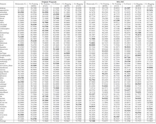
In this subsection we compare the modified versions of the selected self-labeled methods (within SEG-SSC) with the original ones, focusing on the results obtained on the 55 standard classification data sets and a labeled ratio of 10%. We analyze the transductive and inductive accuracy capabilities of these methods. Both results are presented in Tables V and VI, respectively. In these tables, we have specified the base classifier between brackets for Tri-Training and Co-Bagging algorithms. The best result of each row has been highlighted in bold face.

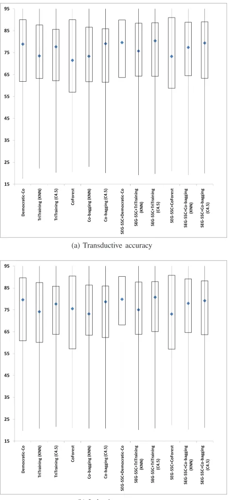
Aside from these tables, Figure 4 depicts two box plot representations of the results obtained in transductive and inductive settings, respectively. With these box plots we show a graphical comparison of the performance of the algorithms, indicating their most important characteristics such as the median, extreme values and spread of values about the median in the form of quartiles (Q1 and Q3).

Observing these tables and the figure we can appreciate differences between each of the original proposals and the improvement achieved by the addition of synthetic examples. Nevertheless, the use of hypothesis testing methods is manda-tory in order to contrast the results of a new proposal with

(a) Transductive accuracy

[image:8.612.322.559.50.564.2]

(b) Inductive accuracy

Fig. 4. Box plot of transductive and inductive accuracy rates. The boxes contain 50% of the data (Q1 to Q3), blue points are the median values and the lines extend to the most extreme values

several comparison methods. The aim of these techniques is to identify the most relevant differences found between methods, which is highly recommended in the data mining field [29]. To do this, we focus on the Wilcoxon signed-ranks test [61] because it establishes a pairwise comparison between methods. In this way, we can see if there are significant differences between the original and modified versions. More information about this test and other statistical procedures can be found at http://sci2s.ugr.es/sicidm/.

(9)

TABLE V

TRANSDUCTIVE ACCURACY RESULTS OVER STANDARD CLASSIFICATION DATA SETS.

Original Proposals SEG-SSC

Datasets Democratic-Co Tri-Training Tri-Training Co-Forest Co-Bagging Co-Bagging Democratic-Co Tri-Training Tri-Training Co-Forest Co-Bagging Co-Bagging

(KNN) (C4.5) (KNN) (C4.5) (KNN) (C4.5) (KNN) (C4.5)

abalone 19.7700 22.1300 20.2800 20.5500 22.9200 20.1100 18.6274 19.1120 19.6966 20.8546 19.2365 19.9401 appendicitis 80.6000 78.1400 82.7300 81.9000 80.3700 82.2600 80.1273 79.6511 80.3736 80.1847 79.4376 81.3013 australian 82.6800 79.0200 82.7700 82.4900 82.0200 81.3200 83.2558 80.7156 80.8587 83.1306 80.6082 80.5546 automobile 32.8500 45.6100 37.7200 41.5600 36.9300 35.1900 43.8713 45.1214 39.0806 41.3491 45.3764 35.4917 banana 84.2700 86.9500 85.1000 53.9400 87.6300 85.7200 85.9003 86.7179 86.7622 54.9849 86.8274 86.9113 breast 70.2000 69.3400 68.6900 71.4800 69.8400 68.9500 71.0801 68.6319 68.3242 69.4731 68.9862 67.7848 bupa 54.2800 55.7900 58.5700 59.4700 55.3100 59.8900 58.1093 56.8213 58.6070 61.1814 56.6096 59.5062 chess 92.0000 79.6200 95.4300 94.3700 81.4600 95.0800 92.0444 82.7566 95.3117 93.9368 84.1663 95.4083 cleveland 53.8000 52.4800 50.2800 51.8500 53.2200 50.8100 54.2972 50.7729 51.3120 53.6428 51.5208 50.8462 coil2000 93.0300 88.2500 93.4300 92.8300 92.3700 93.6300 90.2300 89.0100 92.1800 92.9300 90.2400 90.6400 contraceptive 45.0000 42.0000 47.6600 48.6300 41.7400 47.9700 44.7097 42.4225 48.0525 49.6524 42.8332 46.4188 crx 84.6100 80.8500 84.8100 82.7200 82.7300 84.8300 82.3222 80.4531 83.1333 82.6423 82.1320 81.8868 dermatology 88.0000 89.4800 87.6200 89.3000 87.2400 86.9700 90.2394 90.8924 90.2385 91.6161 91.7198 88.8587 ecoli 63.6400 66.4800 65.9200 66.5600 68.1700 65.7000 65.4363 67.1914 64.9134 69.8830 67.3791 63.4947 flare 71.3300 62.9700 71.1600 39.8700 61.9800 71.2700 70.7523 63.7500 70.1389 39.3403 66.8634 68.7963 german 70.1200 66.2100 68.5800 67.8500 68.5200 69.2000 72.0370 68.1605 68.7778 68.1358 69.0000 69.0617 glass 48.7100 51.2600 49.5500 55.2600 47.7900 45.9700 49.8987 54.2011 51.7359 56.3432 53.1702 50.7878 haberman 73.2300 65.5800 71.6200 58.7000 66.8700 71.4500 72.3424 66.1459 71.2583 62.1837 66.6686 68.9213 heart 78.8600 73.4700 75.6600 71.0500 76.6700 73.7000 79.2694 74.3836 74.2009 73.2877 74.3379 75.0228 hepatitis 81.4200 81.4000 81.4200 84.8800 82.5300 81.4200 78.9245 80.2432 78.9000 84.1557 81.5418 79.3906 housevotes 89.8500 89.1000 92.9500 91.3500 89.0500 93.5400 89.6435 89.7856 92.2012 89.6818 89.4874 92.5117 iris 91.6400 92.1300 75.9000 90.1600 92.3000 80.3300 93.9344 94.1803 83.6066 90.8197 94.0164 83.0328 led7digit 60.0500 59.4300 60.3000 62.9400 66.1700 57.3100 61.8272 61.3333 63.5062 63.3580 63.6790 63.1111 lymphography 51.9000 64.7600 58.9600 61.8000 61.0900 57.6200 58.9634 65.4149 59.0391 62.5010 63.0386 54.8241 magic 78.7300 78.0800 82.0100 84.2000 79.8500 83.2700 79.6235 77.7595 82.4028 84.3311 78.0042 81.6811 mammographic 80.4300 73.8900 81.5600 76.6700 76.3300 81.3600 80.8290 75.7620 81.2622 77.4400 77.3973 80.5495 marketing 27.8800 25.6800 28.1500 28.7900 26.6500 27.8300 26.0327 26.2354 27.0427 28.7900 25.6569 26.4127 monk-2 90.1100 70.5700 97.0300 96.0700 68.5400 97.0300 86.7461 72.0527 92.4715 91.2758 76.5598 88.3120 movement libras 17.5200 40.2800 22.4800 30.4800 36.3800 20.9300 28.8276 44.1379 26.9655 32.9310 43.8276 26.7931 mushroom 99.2600 99.5200 99.5100 90.9200 99.2000 99.4700 99.5213 99.6088 99.7049 90.9362 99.5957 99.7705 nursery 89.6300 76.3200 90.3300 37.6600 73.4900 90.2400 89.5509 78.3274 91.5057 37.8782 78.5675 89.2461 page-blocks 90.6000 93.4200 95.4300 95.7900 93.1300 95.3300 93.7309 93.3202 95.5446 95.6912 93.3789 95.1814 penbased 94.7300 97.7400 90.0200 95.5900 96.8200 90.5000 95.6400 98.0345 92.3247 95.9388 98.0155 93.5455 phoneme 78.6000 80.8000 78.0900 80.4700 79.8800 79.0700 79.9137 80.7817 80.6835 81.8896 80.9576 81.0970 pima 71.9600 65.0600 68.2900 68.5500 65.6200 64.4200 70.4932 66.7475 70.6701 69.6090 67.0209 68.0663 ring 88.7200 66.6000 85.0400 88.4400 61.5200 85.8900 94.6296 82.5375 81.7150 81.5349 86.7901 79.1859 saheart 67.4500 63.3900 65.6600 64.3800 65.6300 65.8700 65.9012 64.8068 65.1284 66.2758 65.3412 65.3147 satimage 85.0600 86.0700 82.3000 86.5500 85.9500 82.1500 85.6518 87.8005 84.1478 86.9986 88.1784 84.3185 segment 90.5900 90.0200 90.3700 90.8600 87.6900 90.9800 90.6197 91.6346 91.0150 92.0726 91.5652 91.5438 sonar 64.3100 65.1900 63.8900 69.2100 65.7800 63.0100 70.3383 67.0835 66.3745 71.2210 67.2593 66.9614 spambase 88.1700 82.8400 88.3700 92.1400 83.3700 89.4700 88.7979 85.9357 90.0437 92.6510 86.9667 90.9567 spectfheart 73.0900 69.6300 72.8200 77.7600 73.3700 72.1200 76.2400 73.3690 75.1242 80.2129 74.2972 76.5126 splice 93.4900 66.5700 81.9500 50.3800 69.5400 81.9700 92.7786 79.8181 87.6393 49.5666 81.2926 89.2918 tae 39.6300 40.7600 39.3700 37.8300 40.6000 38.6400 39.9467 41.0862 40.8437 37.1800 42.3864 41.8213 texture 88.2700 94.4200 85.2600 90.7000 93.4100 84.8800 88.7026 96.4669 89.1021 92.6218 96.4916 90.3681 thyroid 94.1500 90.6400 99.1200 98.6100 92.0300 98.9700 96.7147 91.0460 98.0864 97.5103 91.1094 96.6907 tic-tac-toe 69.7600 70.3200 71.0000 61.8500 67.9700 71.4500 70.5093 70.6640 73.0610 62.8186 72.8934 72.6751 titanic 77.1800 74.6000 77.6900 70.9800 67.7400 77.7700 77.5310 74.5973 77.7834 70.8566 75.5737 77.5086 twonorm 97.0300 93.8000 85.9200 91.3300 95.2200 85.9300 97.3390 96.3664 87.0871 92.0938 96.4097 88.1198 vehicle 47.8700 56.9700 60.4800 64.1500 55.6500 59.0200 57.9951 60.7683 62.1831 66.5154 61.7747 62.1973 vowel 40.6700 48.0400 44.9000 51.9800 37.7200 43.6400 50.3616 50.9601 50.9726 54.4140 51.5586 51.9202 wine 93.0700 92.8500 78.9800 87.5200 93.7600 80.9900 95.1475 93.9660 83.9114 91.0536 92.9243 87.4473 wisconsin 96.2400 95.5000 92.5900 93.4800 95.9400 92.9400 96.6413 95.9910 93.9148 95.6295 96.1535 94.9061 yeast 48.9500 46.3300 49.7300 45.8800 45.9300 48.0800 48.0431 49.5750 50.2999 48.3013 49.2672 49.1259 zoo 92.6200 92.2300 75.4100 89.7800 78.4400 75.5800 86.4836 93.7834 88.2045 93.5267 92.8808 90.2835 Average 73.0475 71.4651 72.5611 71.1002 71.0558 72.3462 74.3477 73.0708 73.6259 71.7279 73.6177 73.3147

Wilcoxon signed-ranks test to the transductive and inductive accuracy rates. It shows the rankings R+ and R− values achieved and its associate p-value. Adopting a level of sig-nificance of α = 0.1, we emphasize in bold face those comparisons in which SEG-SSC significantly outperforms the original algorithm.

With these results we can make the following analysis:

• In Tables V and VI we can see that our framework provides a great improvement in accuracy to the self-labeled techniques used in most of the data sets and rarely does it significantly reduce its performance level. On average, the versions that use synthetic examples always outperform the algorithms upon which they are based in both the transductive and inductive phases. In general, the average improvement achieved for one algorithm in the transductive setting is more or less maintained in the inductive test, which shows the robustness of the models. Co-Bagging (KNN) seems to be the algorithm that bene-fits most when it uses synthetic instances, by contrast, SEG-SSC does not significantly increase the average performance of Co-Forest. Comparing all the algorithms,

the best performing approach is SEG-SSC+Democratic-co.

• It is known that the performance of self-labeled algo-rithms depends firstly on the general abilities of their base classifiers [62]. We notice that C4.5 is a better base classi-fier than KNN for the Tri-Training philosophy. However, the Co-Bagging algorithm performs in a similar way with both classifiers. As expected, the results obtained with our framework are also affected by the base classifier. At this point, we can see that those algorithms that are based on KNN offer a greater average improvement.

(10)

SEG-SSC+Tri-INDUCTIVE ACCURACY RESULTS OVER STANDARD CLASSIFICATION DATA SETS.

Original Proposals SEG-SSC

Datasets Democratic-Co Tri-Training Tri-Training Co-Forest Co-Bagging Co-Bagging Democratic-Co Tri-Training Tri-Training Co-Forest Co-Bagging Co-Bagging

(KNN) (C4.5) (KNN) (C4.5) (KNN) (C4.5) (KNN) (C4.5)

abalone 21.0600 20.7200 21.6100 21.0100 20.7700 20.8200 20.3408 20.1730 20.8922 22.3287 20.3636 21.1299 appendicitis 82.1800 73.8200 80.4500 82.2700 74.7300 80.4500 76.5455 75.7273 79.4545 79.2727 74.7273 83.3636 australian 84.4900 80.2900 84.4900 84.0600 81.3000 82.7500 84.3478 80.4348 82.1739 83.0435 81.5942 82.3188 automobile 36.0100 43.0700 38.8900 45.6900 31.0500 33.6600 44.1879 43.5711 40.7375 40.2639 43.9220 42.4181 banana 84.1700 86.8100 84.8100 52.7000 87.3600 85.5300 85.7736 86.4717 86.8868 55.5472 86.6792 86.7736 breast 72.8700 70.8100 72.1600 73.3900 70.9000 72.5200 72.5921 70.4380 71.9036 70.9338 69.0904 68.7853 bupa 51.0400 54.1600 57.4200 58.5100 57.6600 61.1900 61.9745 54.7159 63.2280 58.5091 57.3746 62.5796 chess 91.9900 83.0900 95.7800 94.4000 80.8800 95.4300 91.4895 78.5345 94.9313 93.2094 83.8238 95.7745 cleveland 52.2300 56.6200 47.6100 53.6600 54.9600 53.3500 55.7156 55.9584 51.0575 53.2235 56.0482 50.6689 coil2000 93.2200 87.9500 93.5700 92.9900 92.2700 93.4800 90.1955 88.2800 92.1100 93.1000 90.1500 90.2500 contraceptive 43.5800 42.1600 48.1300 48.5300 41.0700 48.2700 46.0953 41.7549 47.5188 49.6920 42.9100 47.1824 crx 84.9500 80.3400 85.5500 82.0600 81.0200 84.9600 83.6402 79.2744 83.4395 82.0433 81.7268 80.3731 dermatology 87.6000 89.3000 88.1600 90.4700 87.0800 87.6000 89.3233 90.1495 87.6332 90.6976 91.5388 87.3709 ecoli 63.7000 66.7000 65.8500 62.8300 66.7300 65.5800 68.1907 67.2727 65.5437 67.5758 70.2674 65.8556 flare 72.1400 63.8900 71.5800 40.2400 63.2300 71.4000 71.3939 64.4507 70.3624 38.8415 66.8877 68.5779 german 71.6000 66.7000 71.7000 68.6000 68.8000 71.1000 71.7000 68.5000 68.0000 68.6000 68.3000 70.2000 glass 48.6800 59.4100 49.2100 55.8900 48.2400 48.9800 52.7294 57.1968 56.1803 51.6927 54.2606 54.6483 haberman 71.5600 59.7800 70.8800 60.1400 67.9900 71.2200 71.8602 64.7419 69.2043 59.2903 65.3226 65.2688 heart 80.0000 76.6700 71.4800 69.2600 78.5200 70.3700 80.0000 77.0370 72.5926 71.8519 75.9259 71.8519 hepatitis 83.4300 79.6900 83.4300 81.0900 81.1800 83.4300 82.7446 77.3506 81.2673 90.5032 78.4383 77.7403 housevotes 88.9900 89.3900 91.5800 92.1600 90.3600 91.9500 90.2963 89.0168 88.2021 90.8505 90.3950 90.9857 iris 91.3300 92.0000 72.6700 93.3300 93.3300 80.0000 91.3333 93.3333 83.3333 92.0000 92.6667 84.0000 led7digit 61.6000 59.4000 60.4000 63.4000 66.0000 56.4000 59.8000 60.4000 63.0000 62.6000 61.8000 61.2000 lymphography 49.0100 67.8700 61.1800 64.6400 66.0800 59.4800 68.1709 65.2129 65.2829 68.2017 68.8683 61.5182 magic 78.4200 76.7800 82.4500 84.3600 79.8100 83.1900 79.8370 77.1819 82.3554 84.7266 77.9443 81.9821 mammographic 79.6300 76.9900 81.8300 79.4100 77.5800 80.8500 80.6285 76.5328 81.7016 79.6800 78.3287 79.7660 marketing 27.1000 26.2000 26.9400 29.2300 26.9300 27.0600 25.8285 26.7307 27.5396 29.6700 25.8699 27.1754 monk-2 90.7500 64.6000 96.5700 93.9200 67.0700 96.5700 86.4930 64.3084 92.0869 88.8386 77.0660 86.3375 movement libras 19.7200 44.4400 27.5000 31.1100 34.1700 24.1700 29.7222 43.0556 29.4444 32.5000 43.3333 27.2222 mushroom 99.2700 99.4700 99.5500 90.8400 99.0100 99.5400 99.5531 99.5009 99.7678 90.8713 99.4826 99.8040 nursery 89.5100 86.9800 90.3900 38.0900 73.8500 90.0600 88.4568 75.7330 91.3117 37.3148 78.2330 89.1512 page-blocks 90.7700 93.6400 95.6100 95.8500 93.4900 95.6700 94.3714 93.3847 95.6873 95.8699 93.5306 95.3398 penbased 94.7400 98.0100 90.2700 95.5100 96.8200 90.4900 95.8151 98.2351 92.2486 96.1066 98.0441 93.6136 phoneme 78.7400 80.4600 77.7000 80.0700 79.8300 78.8900 79.4957 80.7726 80.7542 81.3837 80.9578 81.1430 pima 69.6700 62.6500 65.6400 66.2700 63.5800 63.4200 68.1074 64.4723 67.7110 68.6167 65.8994 66.9233 ring 87.4100 60.4100 85.4200 88.2300 61.7600 85.8200 94.3784 69.4189 81.5270 80.2568 86.8649 79.1757 saheart 68.1900 62.7700 67.7600 65.5900 64.0800 64.9700 67.9880 63.2239 66.6744 67.1045 65.6059 64.7317 satimage 84.6200 85.2100 82.2400 86.0000 85.6400 82.0500 85.5945 87.0244 83.8226 86.5584 88.0969 84.3355 segment 90.2600 90.7400 90.0000 90.3000 87.0600 91.6000 91.0390 91.8182 91.2554 91.8182 91.7749 91.5584 sonar 60.0500 63.4500 70.1900 75.5000 65.8800 70.1400 71.0714 66.3571 64.8095 73.0476 63.9524 70.0476 spambase 87.7700 81.1000 88.1000 91.8600 83.2700 89.5100 88.0794 82.4662 90.2108 92.6257 86.5782 90.8852 spectfheart 73.7900 69.0500 75.7400 77.5100 73.1100 75.7100 76.7379 74.9858 79.4444 79.3875 79.8291 79.0456 splice 89.7800 77.5900 82.5400 50.6600 69.7500 82.4800 92.2257 65.8307 88.1191 50.0000 81.7555 89.2476 tae 37.7100 40.4200 45.7100 37.7900 42.8700 42.3700 38.4583 38.3750 38.5417 36.4600 39.0417 39.1667 texture 89.4400 95.2400 85.2400 90.6500 94.3100 85.0000 90.9455 96.8182 89.4909 92.3818 96.8182 90.6727 thyroid 93.9300 90.6700 99.1800 98.5800 92.1000 99.0600 94.2917 91.1250 98.1528 97.6528 91.4444 96.8611 tic-tac-toe 69.0000 70.6700 70.8800 59.7100 67.9600 70.3500 71.5154 71.3004 72.0252 59.0833 72.4452 72.7522 titanic 77.5600 74.1500 77.6500 70.6500 67.4800 78.3700 77.6018 74.1512 78.2378 70.5140 75.1940 77.2394 twonorm 96.4500 91.0900 86.1600 89.8900 95.1800 85.9700 96.8919 93.6351 87.0135 90.6216 96.5270 87.8243 vehicle 50.2300 55.2000 61.9400 61.2400 55.5500 60.3000 59.4664 60.6373 61.7129 63.8459 62.4034 62.5266 vowel 41.6200 49.8000 45.2500 52.2200 39.2900 45.5600 49.1919 52.5253 52.2222 54.3434 52.5253 53.0303 wine 94.9300 92.6500 82.0300 85.8800 93.2700 78.6600 95.5229 93.2026 85.9150 91.0131 96.0784 88.7582 wisconsin 96.5000 94.6200 93.1200 93.5800 95.9300 92.8400 96.3694 95.2032 93.7194 94.6063 95.7938 94.7580 yeast 48.8600 47.5100 49.0700 45.6200 46.7000 47.6500 46.5645 50.1383 50.3387 47.4420 50.2091 47.8501 zoo 93.1400 93.4700 71.9200 90.8900 78.3300 74.5600 88.5000 92.7222 86.9167 92.6389 92.7222 87.3889 Average 73.0362 71.7576 72.9669 71.2424 70.9667 72.7782 74.7488 72.0157 73.9217 71.4700 73.7715 73.5845

Training(C4.5) may be considered the best model. • According to the Wilcoxon signed-ranks test, SEG-SSC

achieves that all the methods significantly overcome their original proposals in terms of transductive learning, sup-porting previous conclusions. However, in the inductive phase, we find that Co-Forest and Co-Bagging (C4.5) have not been significantly improved. Even so, they report higher R+ rankings than the original models, which means that they perform slightly better.

TABLE VII

RESULTS OF THEWILCOXON SIGNED-RANKS TEST ON TRANSDUCTIVE AND INDUCTIVE PHASES

Transductive phase Test phase Comparison R+ R− p-value R+ R− p-value SEG-SSC+Democratic-Co vs. Democratic-Co 1086 454 0.0080 1057 428 0.0067 SEG-SSC+Tri-Training (KNN) vs. Tri-Training (KNN) 1371 169 0.0000 995 545 0.0588 SEG-SSC+Tri-Training (C4.5) vs. Tri-Training (C4.5) 1083 457 0.0086 966 574 0.0997 SEG-SSC+Co-Forest vs. Co-Forest 1132 353 0.0008 863 622 0.2970 SEG-SSC+Co-Bagging (KNN) vs. Co-Bagging (KNN) 1201 339 0.0003 1204 336 0.0003 SEG-SSC+Co-Bagging (C4.5) vs. Co-Bagging (C4.5) 966 574 0.0997 943 597 0.1460

C. Experiments on high dimensional problems with small labeled ratio

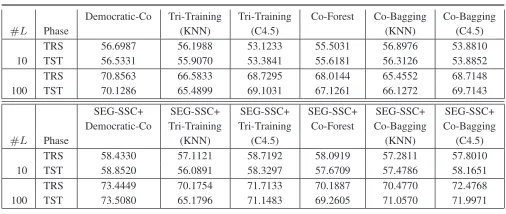
This subsection is devoted to studying the behavior of the proposed framework when it is applied to high dimensional data and a very reduced labeled ratio. Most of the considered data sets (9 of 11) were provided in the book by Chapelle et al. [2], in which the studies were performed using only 10 and 100 labeled instances. We attempt to perform a similar study with the difference that we also investigate the inductive abilities of the models. Furthermore, BBC and BBCsport data sets have been also analyzed in a semi-supervised context with a few number of labeled instances [63].

In the scatterplots of Figure 5 we depict transductive and inductive accuracy results obtained with 10 and 100 labeled data. In these plots, the x-axis position of the point is the accuracy of the original self-labeled method on a single data set, and the y-axis position is the accuracy of the modified algorithm. Therefore, points above they=xline correspond to data sets for which new proposals perform better than the original algorithm.

[image:10.612.56.559.79.477.2]

(11)

30 40 50 60 70 80

Accuracy with the proposed framework

Accuracy of the original proposals Transductive comparison with 10 labeled points

Tritraining (KNN) vs. SE-Tritraining (KNN) Tritraining (C4.5) vs. SE-Tritraining (C4.5) Democratic-Co vs. SE-Democratic-Co CoForest vs. SE-CoForest Co-bagging (KNN) vs. SE-Co-bagging (KNN) Co-bagging (C4.5) vs. SE-Co-bagging (C4.5) y=x

(a) 10 labeled points: Transductive accuracy.

30 40 50 60 70 80

Accuracy of the original proposals Inductive comparison with 10 labeled points

(b) 10 labeled points: Inductive accuracy.

30 40 50 60 70 80

Accuracy of the original proposals Transductive comparison with 100 labeled points

(c) 100 labeled points: Transductive accuracy.

30 40 50 60 70 80

Accuracy of the original proposals Inductive comparison with 100 labeled points

[image:11.612.50.303.558.665.2]

(d) 100 labeled points: Inductive accuracy.

Fig. 5. High dimensional data sets: Transductive and inductive accuracy results

11 data sets considered, including transductive and inductive phases for both 10 and 100 splits.

TABLE VIII

HIGH DIMENSIONAL DATA SETS:AVERAGE RESULTS OBTAINED IN TRANSDUCTIVE(TRS)AND INDUCTIVE(TST)PHASES.

Democratic-Co Tri-Training Tri-Training Co-Forest Co-Bagging Co-Bagging

#L Phase (KNN) (C4.5) (KNN) (C4.5)

TRS 56.6987 56.1988 53.1233 55.5031 56.8976 53.8810 10 TST 56.5331 55.9070 53.3841 55.6181 56.3126 53.8852 TRS 70.8563 66.5833 68.7295 68.0144 65.4552 68.7148 100 TST 70.1286 65.4899 69.1031 67.1261 66.1272 69.7143 SEG-SSC+ SEG-SSC+ SEG-SSC+ SEG-SSC+ SEG-SSC+ SEG-SSC+ Democratic-Co Tri-Training Tri-Training Co-Forest Co-Bagging Co-Bagging

#L Phase (KNN) (C4.5) (KNN) (C4.5)

TRS 58.4330 57.1121 58.7192 58.0919 57.2811 57.8010 10 TST 58.8520 56.0891 58.3297 57.6709 57.4786 58.1651 TRS 73.4449 70.1754 71.7133 70.1887 70.4770 72.4768 100 TST 73.5080 65.1796 71.1483 69.2605 71.0570 71.9971

Given Figure 5 and Table VIII, we can make the following comments:

• In all the plots of Figure 5, most of the points are above the y = x line, which means that, with the proposed framework, the self-labeled techniques perform better than the original algorithms. Differentiating between 10

and 100 available labeled points, we can see that when we have 100 labeled examples, there are more points above this line in both the transductive and inductive phases. We do not discern great differences between the performance obtained in both learning phases which shows that the hypotheses learned with the available labeled and unlabeled data were appropriate.

• Table VIII shows that, on average, the proposed scheme obtains a better performance level than the original ones in most cases, independently of the learning phase and the number of labeled data considered. Attending to the difference between transductive and inductive results, we observe that, in general, SEG-SSC increments both pro-portionally. Nevertheless, there are significant differences between the results obtained with 10 and 100 labeled points.

(12)

use KNN as a base classifier and those that use C4.5. With standard classification data sets, we ascertained that C4.5 was the best base classifier for Tri-Training and performs similarly to KNN for Co-Bagging. These statements are maintained in these domains, where C4.5 performs better. In this study, SEG-SSC+Democratic may be highlighted as the best performing model, obtaining the highest transductive and inductive accuracy results with 10 and 100 labeled examples.

V. CONCLUDINGREMARKS

In this paper we have developed a novel framework called SEG-SSC to improve the performance of any self-labeled semi-supervised classification method. It is focused on the idea of using synthetic examples in order to diminish the drawbacks occasioned by the absence of labeled examples, which deteriorates the efficiency of this family of methods.

The proposed self-labeled scheme with synthetic examples has been incorporated in four well-known self-labeled tech-niques that have been modified by introducing the necessary elements to follow the designed framework. These models are able to overcome the original self-labeled methods due to the fact that the addition of new labeled data implies a better diversity of multiple classifier approaches and fulfills the distribution of labeled data.

The wide experimental study carried out has allowed us to investigate the behavior of the proposed scheme with a high number of data sets with a varied number of instances and features. The results have been statistically compared, supporting the assertion that our proposal is a suitable tool for enhancing self-labeled methods.

Among the used data sets, we have tackled problems related to diverse applications with a high practical interest. For instance, our model can be used to address practical problems such as computer-aided diagnosis, image-classification, spam filtering, etc [21], [47].

There are many possible variations of our proposed semi-supervised scheme that could be interesting to explore as fu-ture work. In our opinion, the use of oversampling techniques with self-labeled techniques is not only a new way to improve the capabilities of this family of techniques, but could also be useful for most of the existing semi-supervised learning algorithms.

REFERENCES

[1] J. Han, M. Kamber, and J. Pei,Data Mining: Concepts and Techniques, 3rd ed. San Francisco, CA, USA: Morgan Kaufmann Publishers Inc., 2011.

[2] O. Chapelle, B. Schlkopf, and A. Zien, Semi-Supervised Learning, 1st ed. The MIT Press, 2006.

[3] X. Zhu and A. B. Goldberg,Introduction to Semi-Supervised Learning, 1st ed. Morgan and Claypool, 2009.

[4] F. Schwenker and E. Trentin, “Pattern classification and clustering: A review of partially supervised learning approaches,”Pattern Recognition Letters, vol. 37, pp. 4 – 14, 2014.

[5] K. Chen and S. Wang, “Semi-supervised learning via regularized boost-ing workboost-ing on multiple semi-supervised assumptions,”IEEE Transac-tions on Pattern Analysis and Machine Intelligence, vol. 33, no. 1, pp. 129–143, 2011.

[6] G. Wang, F. Wang, T. Chen, D.-Y. Yeung, and F. Lochovsky, “Solu-tion path for manifold regularized semisupervised classifica“Solu-tion,” IEEE Transactions on Systems, Man, and Cybernetics, Part B: Cybernetics, vol. 42, no. 2, pp. 308–319, 2012.

[7] A. Blum and S. Chawla, “Learning from labeled and unlabeled data using graph mincuts,” in Proceedings of the Eighteenth International Conference on Machine Learning, 2001, pp. 19–26.

[8] J. Wang, T. Jebara, and S.-F. Chang, “Semi-supervised learning using greedy max-cut,”Journal of Machine Learning Research, vol. 14, no. 1, pp. 771–800, 2013.

[9] A. Fujino, N. Ueda, and K. Saito, “Semisupervised learning for a hybrid generative/discriminative classifier based on the maximum entropy prin-ciple,”IEEE Transactions on Pattern Analysis and Machine Intelligence, vol. 30, no. 3, pp. 424–437, 2008.

[10] T. Joachims, “Transductive inference for text classification using support vector machines,” in Proc. 16th Internation Conference on Machine Learning. Morgan Kaufmann, 1999, pp. 200–209.

[11] P. Kumar Mallapragada, R. Jin, A. Jain, and Y. Liu, “Semiboost: Boosting for semi-supervised learning,” Pattern Analysis and Machine Intelligence, IEEE Transactions on, vol. 31, no. 11, pp. 2000–2014, 2009.

[12] Q. Wang, P. Yuen, and G. Feng, “Semi-supervised metric learning via topology preserving multiple semi-supervised assumptions,”Pattern Recognition, vol. 46, no. 9, pp. 2576–2587, 2013.

[13] I. Triguero, S. Garca, and F. Herrera, “Self-labeled techniques for semi-supervised learning: taxonomy, software and empirical study,”

Knowledge and Information Systems, pp. 1–40, 2014, in press, doi: 10.1007/s10115-013-0706-y.

[14] D. Yarowsky, “Unsupervised word sense disambiguation rivaling su-pervised methods,” in Proceedings of the 33rd Annual Meeting of the Association for Computational Linguistics, 1995, pp. 189–196. [15] A. Blum and T. Mitchell, “Combining labeled and unlabeled data

with Co-Training,” inProceedings of the Annual ACM Conference on Computational Learning Theory, 1998, pp. 92–100.

[16] K. Bennett, A. Demiriz, and R. Maclin, “Exploiting unlabeled data in ensemble methods,” inProceedings of the ACM SIGKDD International Conference on Knowledge Discovery and Data Mining, 2002, pp. 289– 296.

[17] Z.-H. Zhou and M. Li, “Semi-supervised learning by disagreement,”

Knowl. Inf. Syst., vol. 24, no. 3, pp. 415–439, 2010.

[18] G. Jin and R. Raich, “Hinge loss bound approach for surrogate supervi-sion multi-view learning,”Pattern Recognition Letters, vol. 37, pp. 143 – 150, 2014.

[19] U. Maulik and D. Chakraborty, “A self-trained ensemble with semisu-pervised svm: An application to pixel classification of remote sensing imagery,”Pattern Recognition, vol. 44, no. 3, pp. 615 – 623, 2011. [20] A. Joshi and N. Papanikolopoulos, “Learning to detect moving shadows

in dynamic environments,” Pattern Analysis and Machine Intelligence, IEEE Transactions on, vol. 30, no. 11, pp. 2055–2063, nov. 2008. [21] M. Li and Z. H. Zhou, “Improve computer-aided diagnosis with machine

learning techniques using undiagnosed samples,”IEEE Transactions on Systems, Man and Cybernetics, Part A: Systems and Humans, vol. 37, no. 6, pp. 1088–1098, 2007.

[22] L. Breiman, “Bagging predictors,”Machine Learning, vol. 24, pp. 123– 140, August 1996.

[23] N. V. Chawla, K. W. Bowyer, L. O. Hall, and W. P. Kegelmeyer, “SMOTE: Synthetic minority over-sampling technique,” Journal of Artificial Intelligence Research, vol. 16, pp. 321–357, 2002.

[24] I. Triguero, S. Garc´ıa, and F. Herrera, “Differential evolution for opti-mizing the positioning of prototypes in nearest neighbor classification,”

Pattern Recognition, vol. 44, no. 4, pp. 901–916, 2011.

[25] K. V. Price, R. M. Storn, and J. A. Lampinen, Differential Evolution A Practical Approach to Global Optimization, ser. Natural Computing Series, G. Rozenberg, T. B¨ack, A. E. Eiben, J. N. Kok, and H. P. Spaink, Eds., 2005.

[26] J. Alcal´a-Fdez, A. Fernandez, J. Luengo, J. Derrac, S. Garc´ıa, L. S´anchez, and F. Herrera, “KEEL data-mining software tool: Data set repository, integration of algorithms and experimental analysis frame-work,”Journal of Multiple-Valued Logic and Soft Computing, vol. 17, no. 2-3, pp. 255–277, 2011.

[27] A. Frank and A. Asuncion, “UCI machine learning repository,” 2010. [Online]. Available: http://archive.ics.uci.edu/ml

[28] J. Demˇsar, “Statistical comparisons of classifiers over multiple data sets,”

Journal of Machine Learning Research, vol. 7, pp. 1–30, 2006. [29] S. Garc´ıa, A. Fern´andez, J. Luengo, and F. Herrera, “Advanced

(13)

in computational intelligence and data mining: Experimental analysis of power,”Information Sciences, vol. 180, pp. 2044–2064, 2010. [30] M. Li and Z. H. Zhou, “SETRED: self-training with editing,” in

Lecture Notes in Computer Science (including subseries Lecture Notes in Artificial Intelligence and Lecture Notes in Bioinformatics), vol. 3518 LNAI, 2005, pp. 611–621.

[31] S. Dasgupta, M. L. Littman, and D. A. McAllester, “PAC generalization bounds for co-training,” inAdvances in Neural Information Processing Systems 14,Neural Information Processing Systems: Natural and Syn-thetic, 2001, pp. 375–382.

[32] J. Du, C. X. Ling, and Z. H. Zhou, “When does co-training work in real data?”IEEE Transactions on Knowledge and Data Engineering, vol. 23, no. 5, pp. 788–799, 2010.

[33] S. Goldman and Y. Zhou, “Enhancing supervised learning with unlabeled data,” inIn proceedings of the 17th International Conference on Machine Learning. Morgan Kaufmann, 2000, pp. 327–334.

[34] Y. Zhou and S. Goldman, “Democratic co-learning,” in Tools with Artificial Intelligence, IEEE International Conference on, 2004, pp. 594– 202.

[35] Z. H. Zhou and M. Li, “Tri-training: Exploiting unlabeled data using three classifiers,”IEEE Transactions on Knowledge and Data Engineer-ing, vol. 17, pp. 1529–1541, 2005.

[36] L. B. Statistics and L. Breiman, “Random forests,”Machine Learning, vol. 45, no. 1, pp. 5–32, 2001.

[37] M. Hady and F. Schwenker, “Combining committee-based semi-supervised learning and active learning,”Journal of Computer Science and Technology, vol. 25, pp. 681–698, 2010.

[38] M. Hady, F. Schwenker, and G. Palm, “Semi-supervised learning for tree-structured ensembles of rbf networks with co-training.” Neural Networks, vol. 23, pp. 497–509, 2010.

[39] Y. Yaslan and Z. Cataltepe, “Co-training with relevant random sub-spaces,”Neurocomput., vol. 73, no. 10-12, pp. 1652–1661, 2010. [40] T. Huang, Y. Yu, G. Guo, and K. Li, “A classification algorithm based on

local cluster centers with a few labeled training examples,” Knowledge-Based Systems, vol. 23, no. 6, pp. 563–571, 2010.

[41] Y. Wang, X. Xu, H. Zhao, and Z. Hua, “Semi-supervised learning based on nearest neighbor rule and cut edges,” Knowledge-Based Systems, vol. 23, no. 6, pp. 547–554, 2010.

[42] S. Sun and Q. Zhang, “Multiple-view multiple-learner semi-supervised learning,”Neural Processing Letters, vol. 34, no. 3, pp. 229–240, 2011. [43] A. Halder, S. Ghosh, and A. Ghosh, “Aggregation pheromone metaphor for semi-supervised classification,”Pattern Recognition, vol. 46, no. 8, pp. 2239–2248, 2013.

[44] M.-L. Zhang and Z.-H. Zhou, “CoTrade: Confident co-training with data editing,”IEEE Transactions on Systems, Man, and Cybernetics, Part B: Cybernetics, vol. 41, no. 6, pp. 1612–1626, 2011.

[45] I. Triguero, J. A. S´aez, J. Luengo, S. Garc´ıa, and F. Herrera, “On the characterization of noise filters for self-training semi-supervised in nearest neighbor classification,”Neurocomputing, 2013, , in press, doi: 10.1016/j.neucom.2013.05.055.

[46] I. T. Jolliffe, Principal Component Analysis. Berlin; New York: Springer-Verlag, 1986.

[47] C. Deng and M. Guo, “A new co-training-style random forest for computer aided diagnosis,”Journal of Intelligent Information Systems, vol. 36, pp. 253–281, 2011.

[48] Y. Sun, A. K. C. Wong, and M. S. Kamel, “Classification of imbalanced data: A review,” International Journal of Pattern Recognition and Artificial Intelligence, vol. 23, no. 04, pp. 687–719, 2009.

[49] H. He and E. Garcia, “Learning from imbalanced data,”Knowledge and Data Engineering, IEEE Transactions on, vol. 21, no. 9, pp. 1263–1284, 2009.

[50] S. Garc´ıa, J. Derrac, I. Triguero, C. J. Carmona, and F. Herrera, “Evolutionary-based selection of generalized instances for imbalanced classification,”Know.-Based Syst., vol. 25, no. 1, pp. 3–12, 2012. [51] H. Zhang and M. Li, “Rwo-sampling: A random walk over-sampling

approach to imbalanced data classification,”Information Fusion, 2014, in press, doi: 10.1016/j.inffus.2013.12.003.

[52] V. L ´opez, A. Fern´andez, S. Garc´ıa, V. Palade, and F. Herrera, “An insight into classification with imbalanced data: Empirical results and current trends on using data intrinsic characteristics,”Information Sciences, vol. 250, pp. 113 – 141, 2013.

[53] G. E. A. P. A. Batista, R. C. Prati, and M. C. Monard, “A study of the behaviour of several methods for balancing machine learning training data,”SIGKDD Explorations, vol. 6, no. 1, pp. 20–29, 2004. [54] I. Triguero, S. Garc´ıa, and F. Herrera, “IPADE: Iterative prototype

adjustment for nearest neighbor classification,” IEEE Transactions on Neural Networks, vol. 21, no. 12, pp. 1984–1990, 2010.

[55] A. E. Eiben and J. E. Smith,Introduction to Evolutionary Computing. Springer–Verlag, Berlin, 2003.

[56] S. Das and P. Suganthan, “Differential evolution: A survey of the state-of-the-art,” IEEE Transactions on Evolutionary Computation, vol. 15, no. 1, pp. 4–31, 2011.

[57] “BBC datasets,” 2014. [Online]. Available: http://mlg.ucd.ie/datasets/ bbc.html

[58] T. M. Cover and P. E. Hart, “Nearest neighbor pattern classification,”

IEEE Transactions on Information Theory, vol. 13, no. 1, pp. 21–27, 1967.

[59] J. R. Quinlan,C4.5: programs for machine learning. San Francisco, CA, USA: Morgan Kaufmann Publishers, 1993.

[60] D. W. Aha, D. Kibler, and M. K. Albert, “Instance-based learning algorithms,”Machine Learning, vol. 6, no. 1, pp. 37–66, 1991. [61] F. Wilcoxon, “Individual Comparisons by Ranking Methods,”Biometrics

Bulletin, vol. 1, no. 6, pp. 80–83, 1945.

[62] Z. Jiang, S. Zhang, and J. Zeng, “A hybrid generative/discriminative method for semi-supervised classification,” Knowledge-Based Systems, vol. 37, pp. 137–145, 2013.

[63] W. Li, L. Duan, I. Tsang, and D. Xu, “Co-labeling: A new multi-view learning approach for ambiguous problems,” in Proceedings - IEEE International Conference on Data Mining, ICDM, 2012, pp. 419–428.

Isaac Triguero received the M.Sc. and Ph.D. de-gree in Computer Science from the University of Granada, Granada, Spain, in 2009 and 2014, respec-tively.

He is currently researcher in the Department of Computer Science and Artificial Intelligence, Uni-versity of Granada, Granada, Spain. His research in-terests include data mining, data reduction, biomet-rics, evolutionary algorithms and semi-supervised learning.

Salvador Garc´ıa received the M.Sc. and Ph.D. degrees in Computer Science from the University of Granada, Granada, Spain, in 2004 and 2008, respectively.

(14)

Francisco Herrerareceived his M.Sc. in Mathemat-ics in 1988 and Ph.D. in MathematMathemat-ics in 1991, both from the University of Granada, Spain.

He is currently a Professor in the Department of Computer Science and Artificial Intelligence at the University of Granada. He has published more than 240 papers in international journals. He is coauthor of the book ”Genetic Fuzzy Systems: Evolutionary Tuning and Learning of Fuzzy Knowledge Bases” (World Scientific, 2001).

He currently acts as Editor in Chief of the inter-national journals “Information Fusion” (Elsevier) and “Progress in Artificial Intelligence” (Springer). He acts as area editor of the International Journal of Computational Intelligence Systems and associated editor of the journals: IEEE Transactions on Fuzzy Systems, Information Sciences, Knowledge and Information Systems, Advances in Fuzzy Systems, and International Journal of Applied Metaheuristics Computing; and he serves as member of several journal editorial boards, among others: Fuzzy Sets and Systems, Applied Intelligence, Information Fusion, Evolutionary Intelligence, International Jour-nal of Hybrid Intelligent Systems, Memetic Computation, and Swarm and Evolutionary Computation.

He received the following honors and awards: ECCAI Fellow 2009, 2010 Spanish National Award on Computer Science ARITMEL to the “Spanish Engineer on Computer Science”, International Cajastur “Mamdani” Prize for Soft Computing (Fourth Edition, 2010), IEEE Transactions on Fuzzy System Outstanding 2008 Paper Award (bestowed in 2011), and 2011 Lotfi A. Zadeh Prize Best paper Award of the International Fuzzy Systems Association.