University of Twente
EEMCS / Electrical Engineering
Control Engineering
Analysis, optimization and evaluation
of a pipe inspection robot
Harm de Boer
MSc report
Supervisors:
Summary
Gas main inspection in urban areas is very time consuming and expensive. This is why a first robot prototype has been built which can inspect autonomously the pipe network from inside the pipe. However the currently available prototype does not satisfy all the requirements that have to be fulfilled for the first prototype. This master's thesis focuses on a small subset of those requirements e.g. the manoeuvring requirements. The currently constructed prototype is analyzed, optimised and evaluated in relation to the manoeuvring requirements.
First the shortcomings of the existing prototype in relation to the required manoeuvres, were determined. Moving up a slope of 30˚ and through a T-joint is problematic. Also the average speed requirement of 80 mm/s cannot be met. The shortcomings of the existing prototype in relation to these manoeuvres, are analysed for the different prototype modules.
The mechanical construction of the bending module has been optimized to reduce friction, which improved the clamping torque. The maximum necessary clamping torque could not be theoretically determined, because the friction coefficient between the wheel and pipe wall is too high to measure. This high friction coefficient is caused by the deformation of the wheels. However, it can be concluded that the necessary clamp torque that the bending modules can deliver, is sufficient for the different manoeuvres. The overall efficiency of the bending module is low, which is caused by the low clamping speed of approximately (14 mm/s). Using the motor current as clamp torque feedback seems to be a better solution than using the torsion spring elongation. An advantage of using the motor current for control, is that excessive stress on the motors is limited. Also the zero reference is much more accurate and the deviation of the torque as function of the motor current is low. A disadvantage is that only one motor at a time can be used.
From the driving module analysis it can be concluded that the driving motors cannot provide the maximum necessary torque at the nominal motor current. This maximum necessary torque is approximately 131 mNm, while the driving torque at the nominal motor current is approximately 120 mNm. The efficiencies of the driving module are low. These low efficiencies are caused by friction between the gears. The driving speed is approximately 70 mm/s and less above driving torques of 120 mNm. Because the bending speed is also low, the speed requirement of 80 mm/s cannot be met. For driving autonomously, it is recommended to use position/speed control in combination with the motor current control. This prevents excessive stress on the motor.
From the rotation module analysis it can be concluded that the rotation motor can deliver the necessary theoretical torque. During the analysis of the limitations of the current prototype, it has also been determined that the rotation module can practically deliver the necessary rotation torque in the worst case situation. Therefore, the rotation module does not have to be optimized.
Samenvatting
De huidige methoden van gasleidinginspectie kosten veel tijd en geld. Om deze redenen is er een eerste prototype gebouwd van een robot die autonoom van binnenuit het gasleiding netwerk kan inspecteren. Het huidige prototype kan alleen nog niet voldoen aan alle gestelde eisen. Dit onderzoek richt zich op het behalen van een gedeelte van die eisen, namelijk de manoeuvreer eisen. Het huidige prototype is, met betrekking tot het behalen van deze eisen, geanalyseerd, geoptimaliseerd en geëvalueerd.
Eerst zijn de tekortkomingen van het huidige prototype met betrekking tot de gestelde manoeuvreer eisen geanalyseerd. Hieruit kwam naar voren dat het manoeuvreren in een pijp met een helling van 30 graden en het manoeuvreren door een T-bocht problematisch is. Ook de geëiste gemiddelde snelheid van 80 mm/s kan niet worden gehaald. De tekortkomingen van het huidige prototype zijn voor elke module apart geanalyseerd.
De mechanische constructie van de buigmodule is geoptimaliseerd om wrijvingen te verminderen, wat de te behalen klemkracht verhoogde. De theoretisch benodigde klemkracht kan niet worden bepaald omdat de wrijvingscoëfficiënt tussen het wiel en pijpoppervlak te hoog is om te meten. Deze hoge wrijvingscoëfficiënt wordt veroorzaakt door de vervorming van het wielrubber. Het kan wel worden bepaald dat de geleverde klemkracht voldoende is voor de verschillende manoeuvres. De efficiëntie van de buigmodulen is laag, wat mede veroorzaakt wordt door de lage buigsnelheid (14 mm/s). Voor het regelen van de klemkracht, is het beter om de motorstroom te gebruiken voor feedback in plaats van de verdraaiing van de torsieveer. Het voordeel van het gebruiken van de motorstroom voor feedback is dat overbelasting van de motoren kan worden voorkomen. Ook is de klemkoppel spreiding bij een bepaalde motorstroom laag. Een nadeel is dat de buigmotoren niet tegelijk kunnen worden aangestuurd.
Uit de aandrijfmodule analyse kan worden geconcludeerd dat de aandrijfmotoren het benodigde maximale koppel niet kunnen leveren. Dit maximaal benodigd koppel is 131 mNm, terwijl de aandrijfmotoren maar 120 mNm kunnen leveren bij de nominale motorstroom. De efficiëntie van de aandrijfmodulen is ook laag. Dit wordt veroorzaakt door wrijving tussen de tandwielen. De aandrijfsnelheid is ongeveer 70 mm/s bij een koppel van 120 mNm. Omdat ook de buigsnelheid laag is, zal de geëiste gemiddelde snelheid eis van 80 mm/s niet kunnen worden gehaald. Voor autonoom voortbewegen, is het aan te bevelen om een positie/snelheid regeling te combineren met een motorstroom regeling. Dit voorkomt overbelasting van de motoren.
Uit de rotatiemodule analyse kan worden geconcludeerd dat de rotatiemotor het benodigd theoretisch koppel kan leveren. Tijdens de tekortkoming analyse van het huidige prototype, is ook gebleken dat de rotatiemotor ook praktisch het maximaal benodigd koppel kan leveren. Daarom hoeft de rotatiemodule niet te worden geoptimaliseerd.
Preface
With this report I conclude my Master of Science program in Electrical Engineering, which has been a useful addition to my Bachelor education. I would like to thank P. Regtien and E.C. Dertien for their supervising on my work and technical support. I specially would like to thank Tjeerd de Boer for his advice on the report and project planning.
Last but not least, I want to thank my family and girlfriend for their mental support and patience during my study.
Harm de Boer
Table of contents
1 Introduction...8
1.1 Background ...8
1.2 The PIRATE Project ...8
1.3 Assignment...10
1.4 Report Outline ...11
2 Pipe Inspection Robot Overview ...12
2.1 Break Down of the Prototype...12
2.2 Limitations of Current Prototype ...13
2.2.1 Driving Horizontally in a Straight Pipe ...14
2.2.2 Driving up a Slope of 30˚...14
2.2.3 Driving Through a Bend (T-joint/Y-joint) ...14
2.2.4 Take a Diameter Change...15
2.2.5 Average Speed of 80 mm/s ...15
2.2.6 Summary ...15
3 Bending Module Analysis ...16
3.1 Introduction...16
3.2 Basic Bending Module Mechanical Optimizations ...17
3.2.1 Motor Housing and Worm Gear Adjustments ...17
3.2.2 Wheel Adjustments...18
3.2.3 Conclusion ...19
3.3 Calibration and Implementation of Clamp Torque Control...19
3.3.1 Evaluation of Clamp Torque Control with Torsion Spring...19
3.3.2 Evaluation of Clamp Torque Control with Motor Current Feedback ...25
3.3.3 Motor Current Control versus Torsion Spring Control ...31
3.4 Theoretical Necessary Clamping Torque ...32
3.4.1 Mass Measurements ...32
3.4.2 Friction Coefficient Measurements ...33
3.4.3 Conclusion ...35
3.5 Efficiency and Speed Measurements ...35
3.5.1 Efficiency and Speed Test Results ...37
3.5.2 Conclusion ...39
3.6 Bending Module Conclusion...39
4 Driving Module...42
4.1 Introduction...42
4.2 Necessary Driving Torque ...42
4.2.1 Determining the maximum necessary driving torque...43
4.2.2 Conclusion ...45
4.3 Driving Torque, Efficiency and Speed Measurements...46
4.3.1 Driving Torque, Efficiency and Speed test results ...46
4.3.2 Conclusion ...47
4.4 Driving Module Optimizations...47
4.4.1 Gear Train Housing ...47
4.3.2 Gearbox ...48
4.3.3 Reducing Clamping Torque Friction ...48
4.4.2 Driving Control ...48
4.5 Driving Module Conclusion...49
5 Rotation Module ...50
5.1 Introduction...50
5.2 Analysis of Current Rotation Module ...50
5.3 Rotation Module Conclusion...51
6 Conclusions and Recommendations ...52
6.1.1 Manoeuvring Evaluation ...52
6.2 Recommendations...53
Appendix I Test case: Calibration of Clamp Torque Feedback...56
Appendix II Test case: Bending and Driving Efficiency ...66
Appendix III Test case: Calibration of Motor Current as Clamp Torque Feedback...72
Appendix IV Test case: Friction Coefficient...75
Appendix V Test case: Maximum Necessary Driving Torque ...78
1 Introduction
1.1 Background
The national network of gas mains can be divided into a high-pressure (1-8 bar) network for national distribution stretching 20.000 km and a low pressure network (30 mbar to 100 mbar) for local distribution with a length of roughly 100.000 km. The low-pressure net covers most of the urban area's. Therefore this network has the highest priority with regard to risks for public health and safety. Replacement of pipe sections in an urban area is expensive, so it is important to have accurate data on the locations of leaks and damaged pipe sections. Pipes of gray cast iron and white PVC are most likely to cause leakage. Gray cast iron is especially sensitive to corrosion. PVC is sensitive to point-loads (by tools) and tension (bend, stretch) for example caused by tree roots. The main causes of leakage can be summarized as follows: creep, tension, brittleness, impacts, inferior connections, porous rubber sealing and corrosion. There is another issue with the gas mains, besides pipe leakage: the existing network is not well documented. New sections that have been created in the last decade are well documented, but there is not much information available on older sections in the network. Detailed information possibly never existed or got lost in company merges, takeovers and (computer)system changes.
Currently, the low pressure distribution nets are only inspected by conventional leakage searching above ground. This is a labour-intensive process and does not give any information about layout and quality of the pipe, only leaks that can be 'smelled' can be detected. The accuracy of above ground detection is just several meters. By (Dutch) law, every segment of the gas pipe network has to be inspected every 5 years, but with the current methods this is nearly impossible. High pressure mains are already inspected by robotic systems. These systems are hardly full grown autonomous robots, but more passive data loggers. According to Kiwa Gastec(gas technology research), every year 2000 leaks are being found with the conventional leak inspection methods and 6000 leaks are reported by the public. Continuon (network management branch of Nuon energy company) has had 9000 public leak reports in 2005, from which 1000 were false alarm, 2000 leaks were found in house and 6000 were found in the gas distribution network(see [1]).
1.2 The PIRATE Project
Because of the above mentioned problems with the pipe inspection of low distribution nets, Kiwa Gastec and Continuon contacted the University of Twente in 2006 to find a solution which could improve the quality of inspection of the urban pipe network. In cooperation with DEMCON, a project team was then formed called “Pipe Inspection Robot Autonomous Tube Exploration” (PIRATE). The PIRATE project focuses on the development of an automated system, which can inspect the pipe network from inside the pipe. Goal of the project is to design and build a prototype of an autonomous robot platform, which can navigate through a pipe network.
Problem Requirements/Specifications Mechanical Design
Electronic Design
Software Design
First Prototype November 2006 September 2007 October 2007
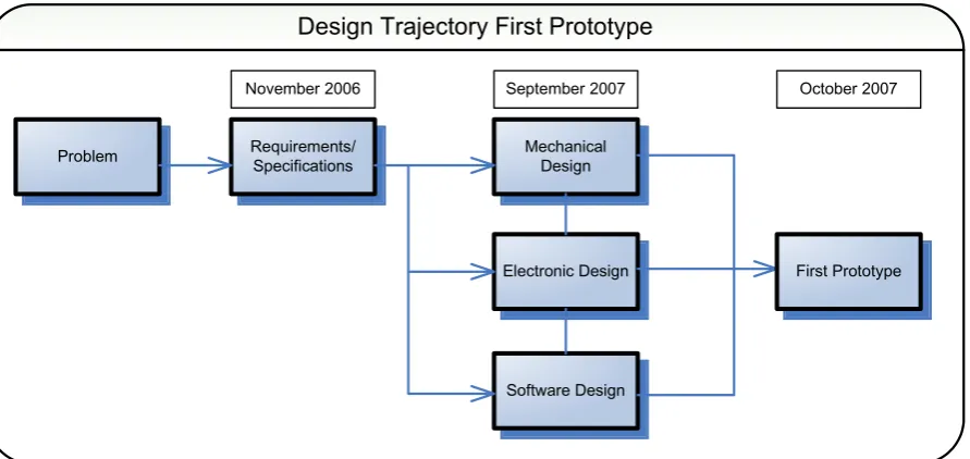
[image:10.595.79.525.71.282.2]Design Trajectory First Prototype
Figure 1.1: First phase design trajectory overview
Because the development of the pipe inspection robot is very challenging, it will be carried out in several phases. Figure 1.1, gives an overview of the executed first phase in the development trajectory. Not all the requirements have to be met in the first phase. For the first phase, the robot should only have to be able to manoeuvre in a pipe network without having to detect leaks and deformations of the gas pipe. The parameters of such a pipe network are shown in table 1.1.
Property Parameterization
Smallest inner diameter 57 mm.
Biggest inner diameter 119 mm.
Maximum inclination of the pipe Angle of ≤ 30˚
Gradual diameter change 57 mm. To 119 mm. Angle ranging from 0˚ to 45˚
Bends Mitered and smooth bends (Angle of ≤ 90˚)
Table 1.1: parameters of the pipe network
Additional requirements on the first phase are:
• The robot should be able to manoeuvre autonomically through a pipe network
• The robot has to communicate wireless with the operator
• Average speed of the robot has to be approximately 80 mm/s
• The robot should have enough power to function for 30 minutes, which should be enough for demonstration purposes.
Not in scope:
• Demands on reliability
• Detections of leaks and deformations of a gas pipe
The second phase in the design trajectory was the design of the mechanical, electrical and software parts. J.J.G. Vennegoor op Nijhuis finished his Master of Science study at the University of Twente with a thesis about the mechanical design of the pipe inspection prototype. The study translates the specifications and demands of the parties involved in the PIRATE project, to a complete mechanical design. A few mechanical concepts are explored and evaluated on feasibility (see [2]).The chosen concept is further detailed and engineered to a production ready design which is shown in figure 1.2.
Figure 1.2: The chosen concept
The electronic and software design is divided in two main parts.
• The first part is the design of the local controllers which control all the different motors separately. The design and implementation of these controllers was part of a Master of science internship at the university of Twente which is performed by J. Ansink (see [3]).
• The second part is the main controller which has to control all the routines of the local controller boards and has to communicate with the operator. This is designed and implemented by E.C. Dertien (see [3]).
All these parts combined, resulted in a first prototype of the pipe inspection robot. It has been build for demonstration purposes and to show the technology to the parties involved and potential investors.
1.3 Assignment
The current prototype which has run through two phases of development, does not satisfy all the requirements that it has to fulfil. This master's thesis focuses on a small subset of those requirements e.g. the manoeuvring requirements.
1.4 Report Outline
In chapter 2 Pipe Inspection Overview, the limitations of the current prototype will be discussed.
In chapter 3, 4 and 5, the different modules of the robot will be evaluated separately. For each module the characteristics are analysed, and possible optimizations are discussed and evaluated.
2 Pipe Inspection Robot Overview
[image:13.595.72.525.210.444.2]
2.1 Break Down of the Prototype
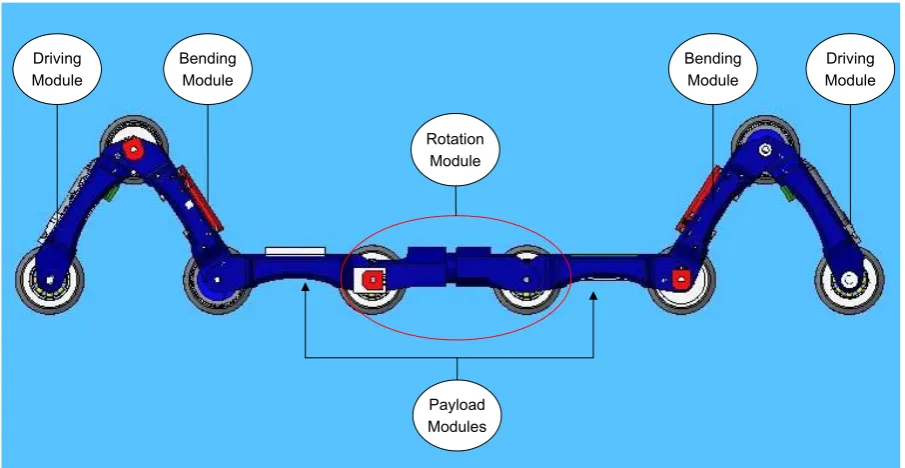
Figure 2.1 shows schematically the current prototype. It consists of five active modules and two passive modules, each having one of four different specific functions. These modules will be introduced shortly.
Bending Module
Rotation Module Driving
Module
Payload Modules
Driving Module Bending
Module
Figure 2.1: Schematic representation of current prototype
• Bending module
Two bending modules are present at the rear and front side of the prototype. The function of the bending module is to clamp and orientate the robot in the pipe. The clamping is necessary for providing sufficient traction to the wheels. The bending module is connected to the drive module and to the payload module. The driving module forms together with the bending module the clamping module.
• Driving module
Two driving modules are present at the rear and front side in the prototype. The function of the driving module is to actuate the robot inside the pipe.
• Rotation module
One rotation module is present in the middle of the prototype. The function of the rotation module is to orientate the robot in a different direction. It rotates one half of the robot with respect to the other half.
• Payload modules
The two passive payload modules are used to fit the main controller and batteries in the robot.
Figure 2.2: schematically overview of electronic infrastructure
The control of the robot is based on distributed control, as can be seen in figure 2.2. The main controller performs the high level control, and the local controllers perform the local feedback control of the different motors for bending, driving and rotating.
The main controller board consists of an ARM7 processor, a 3D acceleration sensor (to determine the orientation of the robot), a memory card slot and a radio module for external (wireless) communication. The current pipe inspection prototype communicates via a RS232 interface with the operator. All the commands of the operator are passed through by the main controller to the different local controllers. The communication between the main controller and the local controllers is based upon I2
C.
The local controller consists of an AVR ATmega 168 microcontroller, two H-bridges and sensor interfaces. It provides the following functionalities:
• Control the motors with a PID feedback loop. The feedback consists of information from different sensors. The controller output is a PWM value, which is send to the bridge. When the control loop is disabled, PWM values are sent directly to the H-bridge.
• Analog to digital conversion (ADC) for different sensor interfacing
• Interface for communication with the main controller
More detailed information about the local and main controller can be found in respectively [3] and [4].
2.2 Limitations of Current Prototype
As mentioned in the introduction, the current constructed pipe inspection robot does not meet all the manoeuvring requirements for the first prototype. After performing some small tests with the prototype, the compliance to the following manoeuvring requirements are discussed:
1. Plain driving in horizontally position a straight pipe 2. Driving up a slope of 30˚
3. Driving through a bend (T-joint/Y-joint) 4. Take a diameter change
2.2.1 Driving Horizontally in a Straight Pipe
For most of the time, the robot will drive horizontally in a straight pipe. For this manoeuvre, the robot is clamped horizontally inside the pipe by using the rear and front bending module. Both modules are providing the traction to the wheels, which are actuated by the driving modules. The necessary driving and clamping torque for this manoeuvre can be delivered by the modules, so this requirement is met.
2.2.2 Driving up a Slope of 30˚
To drive up a slope, it is assumed that the robot will be clamped again horizontally inside the pipe by both bending modules and that the actuation is delivered by both driving modules. For this manoeuvre, the traction force to the wheels has to be larger than for driving in a straight pipe (see [2]). This necessary traction when driving up a slope of 30˚, cannot be
delivered by the bending modules. The wheels are slipping when they are actuated. This requirement is not met.
2.2.3 Driving Through a Bend (T-joint/Y-joint)
Driving through a bend is a difficult manoeuvre. In figure 2.3 this manoeuvre is schematically shown for a T-joint which is the most difficult.
Figure 2.3: Schematic overview of manoeuvring through a T-joint
Figure 2.3 shows a top view of the pipe, where the robot approaches the T-joint driving sideways. The sequence is as follows:
• The robot approaches a T-joint
• After the front driving module has reached the opposite wall, the front actuated wheel looses contact with the wall. The rear module now has to deliver the traction and actuation to push the front module against the opposite wall
• The front module bends into the T-joint and initially builds up traction in the new pipe segment
• As the front module moves further into the new pipe segment, the robot clamps itself again in the new pipe-segment
The delivered clamping torque is insufficient to take these manoeuvres. It cannot provide enough traction when driving sideways and when only one module has to deliver the traction. This part of the requirement is not met.
For approaching the T-joint sideways, the rotation module has to rotate the robot. A rotation sequence includes the following steps:
• First one of the bending elements increases the clamping torque and the other decreases the clamping torque until the wheels loose contact with the wall
• Now the bending module with the highest clamping torque decreases the torque and the other one increases the torque
• Finally the rotation motor turns to the neutral position
Rotation of the robot inside the pipe is possible with the current prototype. This part of the requirement is met.
2.2.4 Take a Diameter Change
Taking a diameter change does not require specific demands on the delivered torques. The robot should be able to adjust the angle between the driving and bending module while passing through the diameter change, in order to keep the wheels in contact with the wall all the time. With the current prototype, this can be accomplished, so this requirement is met.
2.2.5 Average Speed of 80 mm/s
In all manoeuvres, the average speed should be 80 mm/s. This requirement cannot be met by the current prototype. This was already concluded during the mechanical design (see [2]). This requirement is not met.
2.2.6 Summary
An overview of the evaluation of the current prototype with respect to the manoeuvring requirements, is shown in table 2.1.
Requirement
Drive horizontally in straight pipe
;
Rotate the robot
;
Drive up a slope of 30˚
:
Drive through a bend (T-joint/Y-joint)
:
;
Take a diameter change
;
Average speed of 80 mm/s
:
Table 2.1: overview of evaluation
3 Bending
Module
Analysis
3.1 Introduction
In this chapter the analysis of the bending module will be discussed. In the prototype there are two bending modules present as can be seen in figure 2.1. The function of the bending module is to clamp and orientate the robot in the pipe. This clamping is schematically shown in figure 3.1.
ß
L1 r
Fclamp2 Fclamp2
r
Fclamp
D1
D2
To
p V
iew
Figure 3.1: Schematic top view of a bending module clamped inside a pipe
Input to the bending module is a Pulse Width Modulated (PWM) signal which controls the power to the bending motors. The bending module contains two Faulhaber 1016 motors to be able to set two bending angles (ß) and a torque between the bending module and the two connected modules. With this clamping torque, the robot can clamp itself inside the pipe with a certain clamp force (Fclamp). The motors can each deliver a nominal torque of 0.48 mNm. To increase the clamping torque, a transmission gearbox is introduced between the motor and the actuated wheel. The construction of the gearbox is depicted in figure 3.2. With the gearbox a total transmission ratio of 1:5486 with an estimated efficiency of 21% can be reached. This will theoretically provide a clamping torque of 563 mNm at the nominal motor current.
Figure 3.2: Bending module transmission
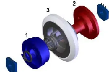
potentiometers. The potentiometers are connected to a torsion spring element (which is located in the actuated wheels) in order to translate the clamp force to a potentiometer position. Figure 3.3 represents the assembly of the wheels.
Figure 3.3: Assembly of wheels with torsion spring
This assembly consists of the wheel with a rim and two bodies with a torsion spring in between. The torque applied by the bending module is passed on to body number one and then again transferred to body two via the torsion spring in between body number one and two. Body number two is connected to the adjacent module. If a torque builds up between two modules, the spring will elongate. This elongation is a measure for the build up torque and is measured using a potentiometer that is connected to the shaft of body two and the housing of body one. Finally the two bodies are made out of aluminium bronze to function as sliding bearing for the wheel that surrounds the bodies. The bending angle and clamp force information (potentiometer reading) can be used to control the bending module.
In chapter 2.2 it has been determined that the bending module cannot practically deliver the necessary clamping torque to accomplish the required manoeuvres. To analyse why the bending module cannot deliver the necessary clamping torque, different tests need to be performed to determine the theoretical necessary and the practically delivered clamping torque. After performing some small tests, it has been determined that the bending module suffers a lot from friction. The clamping torque was approximately 20% of what it theoretically could be (563 mNm).
In the following chapters, the different areas of improvement are discussed.
3.2 Basic Bending Module Mechanical Optimizations
Before performing tests on the bending module performance, some basic mechanical imperfections have been addressed. These imperfections are described in the following subchapters.
3.2.1 Motor Housing and Worm Gear Adjustments
After examining the worm gear itself, it could be seen that this gear is assembled with a slight excentricity. It was also noticed that the bearing that is placed at the end of the worm gear has a larger diameter than the motor and worm gear (which have the same diameter). This causes the worm wheel to be pushed extra against the motor housing. By enlarging the diameter by a couple of micrometers at the ends of the motor housing, the motor, worm gear and end bearing can be placed again in a straight line. These optimizations reduce the total amount of friction of the bending module.
Figure 3.4: Motor housing of the bending module
Besides the mentioned optimizations, the motor housing material (bronze) appears to be not stiff enough. For fixing the bending motors and gears inside the motor housing, screws on the top of the motor housing need to be tightened. However, because the material is not stiff, the motor housing deforms slightly. This makes it difficult to place the motor and gears in a straight line. For this reason it is recommended to choose another material for the motor housing.
3.2.2 Wheel Adjustments
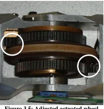
Another part that causes unwanted friction is the actuated wheel. To this wheel, one or two gears are connected which make contact with other gears (from the bending and driving module) as can be seen in figure 3.5 (marked with circles). These gears make also contact with the wheel rubber, which causes additional friction. To eliminate this friction, one millimetre from the sides of the wheel rubber is removed. As can be seen, this adjustment does not decrease the wheel surface which makes contact with the pipe wall.
Figure 3.5: Adjusted actuated wheel
3.2.3 Conclusion
The bending module can theoretically deliver a clamping torque of 563 mNm, but in practice this value is not reached. The bending module is not able to comply to the manoeuvring requirements. Different imperfections of the construction can be pointed out as reason for not reaching the theoretical clamping torque:
• Worm-gear bearing does not fit perfectly in motor housing (friction between worm-gear and motor housing)
• Imperfect attachment worm-gear and motor (slight eccentricity) (friction between worm-gear and motor housing)
• Motor housing deforms when assembled (friction between worm-gear and motor housing)
• Transmission gear contact with wheel rubber (friction between wheel rubber and transmission gear)
Except for the motor housing deformation, all other imperfections have been resolved. The motor housing deformation has not been addressed due to time-constraints. The exact gain in clamping torque due to these improvements has not been determined, but improvements in clamping torque were evident.
The improved construction has been used as basis for further analysis described in this document.
3.3 Calibration and Implementation of Clamp Torque Control
For the different tests that need to be performed, clamping torque control has been implemented and calibrated. Two methods of determining the clamp torque will be discussed.
3.3.1 Evaluation of Clamp Torque Control with Torsion Spring
3.3.1.1
Introduction
As already mentioned in chapter 3.1, the elongation of the torsion spring is a measure for the clamping torque and is measured using a potentiometer. The potentiometer delivers an analogue value which is converted to ADC signals, used as a feedback signal for the clamp torque control.
For the calibration of the clamping torque, two values are relevant:
• The torque per ADC bit (Torque/ADC ratio)
• The ADC value of the bending module when it is not bended (the spring is not elongated in this position)1
Both values are determined through the clamping torque calibration test, of which the setup is shown in figure 3.6.
Figure 3.6: test setup for clamp torque calibration
In the figure, the clamping module slides sideways with the middle axis and the lower wheels in a groove, which has the same length as the largest pipe diameter (119 mm). The friction that is caused by this sliding is negligible. For easy calculation, the bending is performed sideways to eliminate the gravitational force. To the bending module, a spring scale is attached to measure the applied clamp force. This spring scale has a range of 0 to 10 Newton. (For more detailed information about the test, see Appendix 1).
The torque/ADC ratio is measured by applying a force of 2 to 8 Newton with steps of 1 Newton. This limited clamp force is necessary to avoid stressing the torsion spring, which can handle a maximum clamp torque of 900 mNm. The ADC values at the different applied clamping forces are read, and the length of the arm of the momentum is measured. This experiment is performed ten times to have a more accurate ADC value. The clamping torque can then be determined with formula (1). Here the applied force is multiplied with the measured arm of the momentum (r):
(1)
τ
clamp=
F
clampi
r
The torque/ADC ratio can then be determined with formula (2):
(2)
11
/
n nn n
T
T
ADC ratio
ADC
ADC
τ
++
−
=
−
Here Tn and ADCn are for example the clamping torque and ADC measurements for a clamp force of 1 Newton and Tn+1 and ADCn+1 the torque and ADC measurement for a clamp force of 2 Newton. To determine whether after reassembling the clamping module the torque/ADC ratio and setpoint remains the same, the entire experiment is repeated one time after taking apart and reassembling the clamping module.
Besides the Torque/ADC ratio measurements, the ADC value of the bending module at a clamp force of 0 Newton is also measured. This value will be the zero point of the clamping torque feedback.
Because the torsion spring (see chapter 3.1) has a linear characteristic, the Torque/ADC ratio is expected to be approximately constant for all applied clamp forces and is calculated as follows:
(3)
resolution ref maxin
U
U
bit resolution
θ
θ
=
i
i
In this formula,
U
refis
the reference voltage of the potentiometer (1.1 V, see [3]),U
in is the input voltage of the potentiometer (3.3 V, see [3]),θ
max is the maximum angle (333˚, see [3]) and the bit resolution is 1024 (see [3]). This gives an angle resolution of 0.1084˚According to [2], the maximum torque that the torsion spring can handle (Tmax_spring) is 900 mNm at a deflection of 24˚ (θmax_spring). The maximum ADC output can be calculated with
formula (4, see [3]), using the angle resolution calculated in the previous step (formula 3):
(4)
max max_spring221
resolution
ADC
θ
θ
=
≈
According to [3], the torque/ADC ratio can be determined with formula (5):
(5)
max_max
900
/
4,1
221
springT
ADC ratio
mNm
ADC
τ
=
=
≈
This means, that one ADC bit should correspond to a clamping torque of 4,1 mNm.
3.3.1.2
Test results
The test results for the front and rear bending module are respectively presented in table 3.1 and 3.2. (More detailed test results can be found in appendix I)
First measurement After reassembling
Clamp Force (N)
μ
σ
μ
σ
2 to 3 4.1 1.2 6.3 1.6
3 to 4 4.1 0.7 3.7 0.8
4 to 5 3.8 0.5 4.2 0.9
5 to 6 5.2 1.5 6.0 2.3
6 to 7 5.0 1.5 19.6 17.9
7 to 8 5.9 1.5 16.6 12.8
Table 3.1: standard deviation and mean of all measured ratio’s for the rear bending module
First measurement After reassembling
Clamp Force (N)
μ
σ
μ
σ
2 to 3 4.9 1.5 3.8 0.6
3 to 4 6.3 1.8 4.4 1.2
4 to 5 4.1 0.5 4.0 1.6
5 to 6 4.2 0.3 6.9 4.4
6 to 7 4.1 0.9 4.4 1.3
7 to 8 6.6 3.4 19.4 16.1
Table 3.2: standard deviation and mean of all measured ratio’s for the front bending module
and if the standard deviation would be small. As can be seen in table 3.1 and 3.2, the following can be observed:
• there is clearly a non-linear relationship between the applied clamp forces and the measured Torque/ADC ratio’s and can vary from 3.7 to 19.6 for increasing clamp forces, which is very large
• there is a spread in the measured Torque/ADC ratio which can get very large. The spread in measured ratio’s is smaller for low applied clamp forces than for high applied clamp forces
• the measured Torque/ADC ratio’s for both bending modules after reassembling differ a lot
The third observation is due to the impossibility to reassemble the wheel construction exactly in the same position as before the disassembly. For this reason it is not possible to determine a fixed setpoint for the clamp torque feedback.
Both first observations (the non-linear relation and the measured spread in Torque/ADC ratio) are mainly caused by measurement noise, bearing friction and backlash effects that are present in the bending modules.
3.3.1.3
Measurement Noise Effect
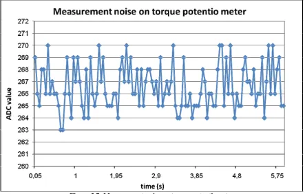
[image:23.595.77.521.434.716.2]To determine the contribution of the measurement noise to the spread in Torque/ADC ratio, a test has been carried out on the ADC value stability. During this test, the motors are active (to create a active/loaded scenario) and the potentiometer is kept at a fixed position (i.e. value does not change). The result is depicted in figure 3.7.
Figure 3.7: Measurement noise on torque potentiometer
of the measured Torque/ADC ratio spread. This noise does not depend on the state of the motor (active or inactive)
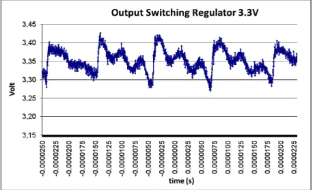
[image:24.595.70.529.424.702.2]The measurement noise appears to be caused by the max1759 switching regulator, which converts a battery voltage of 3.7V to a voltage of 3.3V. This 3.3V is the input voltage of the potentiometer (
U
in in formula (3)). Figure 3.8 shows the schematics of this switching regulator.Figure 3.8: Schematic of the max1759 switching regulator
As can be seen in figure 3.8, there is a low pass filter at the output of the switching regulator. This low pass filter is used to produce a smooth output voltage. However, figure 3.9 shows that this output voltage is not stable and has a saw tooth shape.
Figure 3.9: Output of the switching regulator
the current sense amplifier datasheet (see [6]) it is recommended to use 0.33 μF for the C413 capacitor. Because of better availability, currently a 0.47 μF capacitor is used.
3.3.1.4
Bearing Friction Effect
In the actuated wheels of the prototype, a non ideal bearing is used that does not eliminate parasitic friction (friction caused by the different ways the bearing surfaces can rub against each other). Using pre-stressed bearings in the wheel would be a better solution but there is not much space for these bearings. In [2], some experiments were performed with different bearings, but because of the limited space in the wheel and the limited time available, the current bearings are chosen.
This effect contributes to the non-linearity of the torque/ADC ratio.
3.3.1.5
Backlash Effect
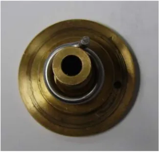
[image:25.595.216.380.379.534.2]The torsion springs in the wheels are not assembled properly. The springs are not centred correctly around the wheel axis as can be seen in figure 3.10. This causes extra friction. Also the spring ends are not well fixed, this causes the backlash present in the bending module. It is difficult to produce torsion springs which do not have any deformation. It is difficult to reshape these springs in the proper form. This effect contributes to the non-linearity in torque/ADC ratio.
3.3.2 Evaluation of Clamp Torque Control with Motor Current Feedback
3.3.2.1
Introduction
As the method for clamping torque determination by torsion spring elongation is not deterministic enough, an alternative method for determining the clamping torque has been considered.
This alternative method uses the motor current to determine the clamp torque. Because there is theoretically a linear relationship between the motor current and the output torque of the Faulhaber motors, this could be a useful torque feedback.
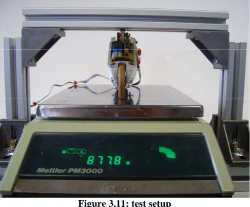
[image:26.595.171.425.306.516.2]In order to decide whether the motor current can be used to determine the clamp torque, tests have been carried out. The “clamp torque/motor current” characteristic and the spread between measured torques at a certain motor current has to be determined. The test setup is shown in figure 3.11. It consists of a balance and a construction where the “pipe wall” can be simulated with. (For more detailed information see appendix III)
Figure 3.11: test setup
During the test, an external power supply delivers 6 volt to the prototype. For a few motor currents from 0.12 Ampere up to a current of 0.17 Ampere (0.16 Ampere is the nominal current), the clamp torque is measured.
The clamp torque is calculated with formula (6):
(6)
τ
clamp=
m g r
i i
In formula (6), m is the mass that the balance indicates when the bending module clamps itself at a certain motor current between the balance and “pipe wall”, g is the gravitational acceleration and r the arm of momentum.
3.3.2.2
Test Results
mm and 119 mm.). For each motor current at a certain pipe diameter, the achieved clamp torque is measured ten times to determine the clamp torque spread.
Table 3.3 shows the measured mean torques and the standard deviation at the applied motor currents and pipe diameters for the front bending module.
Diameter 57 mm. Diameter 119 mm. I (Ampere)
µ (mNm) σ (mNm) µ (mNm) σ (mNm) 0.12 508 18 392 36
0.13 548 21 484 32
0.14 569 26 527 20
0.15 613 20 570 18
0.16 622 14 586 13 0.17 628 12 609 13
Table 3.3: measured mean torque and standard deviation of front bending module
Table 3.4 shows the measured mean torques and the standard deviation at the applied motor currents and diameter for the rear bending module.
Diameter 57 mm. Diameter 119 mm. I (Ampere)
µ (mNm) σ (mNm) µ (mNm) σ (mNm) 0.12 548 13 550 26
0.13 554 12 579 16
0.14 575 9 640 18
0.15 601 10 663 17
0.16 618 12 681 15 0.17 654 12 684 14
Table 3.4: measured mean torque and standard deviation of rear bending module
As can be seen in table 3.3 and 3.4, the following can be observed:
• there is clearly a non-linear relationship between the applied clamp forces and the motor current
• there is a spread in the measured torque as function of the motor current
• there is a difference in the torque/current relation for the different pipe diameters, but not as significant as would have been expected. Expected was that the largest pipe diameter would give the larger torque for the same current. Because the gear that is directly connected to the actuated wheel is assembled with some eccentricity, the front bending module has a larger clamp torque at a smaller diameter.
• it is noticed that both bending modules have a different motor current / clamp torque characteristic. Therefore, the controllers of both modules have to be given separate setpoints to deliver the same clamp torque.
Furthermore, it has been observed that the clamping torque/motor current ratio remains rather constant after disassembling/reassembling of the construction.
3.3.2.3
Complexity of Using Motor Current Feedback
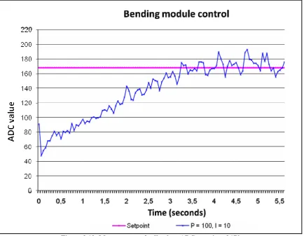
measurements (as depicted in figure 3.12, where the ADC value represents the motor current).
[image:28.595.82.517.123.460.2]
Figure 3.12: Motor current feedback at ADC setpoint of 170
Because the motor current measurement suffers from noise, the PID control will be difficult to configure with the Ziegler and Nichols rules (see [4]), as it is not possible to determine the oscillation frequency, considering only proportional control. Therefore, the PID gains have to be determined experimentally.
Because there is enough damping in the mechanical construction of the prototype, only the proportional and integral action in the PID controller are used. The integral action is used to decrease the stationary error. The PI gains are experimentally tuned to get a smooth step response with minimal overshoot. The PI gains are equal to Kp = 100 and Ki = 10. Figure 3.12 represents the result of the motor current feedback (ADC value) when the setpoint is 170. Note that in order to have a stable control after reaching the setpoint, a small threshold is implemented in the local controller software to suppress the influence of the measurement noise.
As can be seen in figure 3.12 does the motor feedback control have, besides the first few milliseconds, a more or less smooth step response. In the first few milliseconds a peak motor current is seen as consequence of the motor being started.
Figure 3.13: high-side current sensing schematic
[image:29.595.73.505.407.706.2]For the current sensor a high-side current amplifier (MAX4372T) to measure the current at the high-side of the H-bridge is used, because with the H-bridge that is chosen for the local controller it is not possible to do a reliable low-side current sensing. All the current that is used by the motor will flow through the high-side of the bridge without any leakage. To be able to measure the current, a series resistor (R202) is needed that converts the current into a small voltage across the series resistor. This voltage will be amplified with a factor of 20 by the high-side current amplifier and filtered (low pass filter R203 and C208) afterwards to reveal a cleaner voltage for the micro controller AD-converter.
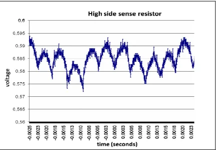
Figure 3.14 and 3.15 shows the measured signal at respectively the high side and low side of resistor R202.
Figure 3.14: Voltage at the high side sense resistor
Figure 3.15: Voltage at the low side sense resistor
Figure 3.16: Amplifier output at 50% duty cycle
As can be seen in figure 3.16, is the output of the current amplifier a block signal with some small noise. After the filtering a clean voltage is expected, however as can be seen in figure 3.17 has the filtered output voltage a saw tooth shape with a frequency of 2 kHz and a large amplitude of almost 0.3 Volt.
[image:31.595.86.511.438.740.2]The -3 dB point of the low pass filter is chosen to be approximately 160 Hz. Because the high frequencies are not suppressed enough, this low pass filter has to be adjusted.
[image:32.595.89.514.161.440.2]This filtered voltage is then send to the AD converter. This explains the noise in the ADC measurements. The motor current measurement noise at 50% and 100% duty cycle after the AD conversion is shown in figure 3.18.
Figure 3.18: Measured ADC motor current value at 50% and 100% duty cylce
As can be seen in figure 3.18, the maximum measurement noise at 50% is approximately 70 ADC values and for 100% duty cycle 20 ADC values. This corresponds to a motor current of respectively 0.06 and 0.02 Ampere.
3.3.3 Motor Current Control versus Torsion Spring Control
From the evaluation of the torsion spring feedback, it can be concluded that it is difficult to determine the clamping torque through this method:
• the torque/ADC ratio is not constant and has a large spread, caused by mechanical and electrical deficiencies
• the zero reference is not deterministic due to the sensitive assembly of the construction
Using the motor current as clamp torque feedback seems to be a better solution. An advantage of using the motor current for control, is that the zero reference is much more accurate and the deviation of the torque as function of the motor current is low.
limit (high start up motor current), this limit is set high. By only controlling the clamp torque with the elongation of the torsion spring, no care can be taken to prevent the motors from being stressed. By controlling the torque with the motor current, both the torque and the current to the motor is controlled.
A disadvantage of controlling the clamping torque with the motor current, is that just one motor at a time can be used because only the total motor current can be measured. For driving autonomously, also position control (angles that are measured with potentiometers) have to be used in combination with the motor current control. This is because the bending motor that is actuating wheel between the bending module and payload module, will clamp further than required. That is why the position control need to be the high level control. When the position is reached, the bending motor should be shut down.
3.4 Theoretical Necessary Clamping Torque
The theoretically necessary clamping torque will be analysed in this section, in order to determine whether the chosen motors and gears can theoretically deliver this torque. During the detailing of the chosen pipe inspection robot concept, the calculation of the maximum necessary clamping torque is carried out (see [2]).
In the calculations in [2], formula (7) is used for calculating the necessary clamping torque per bending module:
(7)
1
8
clampm g
r
τ
μ
=
i i
i
In this formula represents
τ
clamp the necessary clamping torque, r a distance called the arm of the momentum (see 3.1), m the mass of the robot, g the gravitational acceleration and μthe friction coefficient between the wheel and the pipe wall. With this formula it has been determined that a clamping torque between 800 and 1000 mNm. should be sufficient for driving in the worst case situation. This worst case situation is estimated to occur when the robot is driving sideways up a slope of 30˚ in the smallest pipe (57 mm).
This determined necessary clamping torque cannot be provided by the bending motors without stressing them, because they can theoretically deliver only 563 mNm at the nominal motor torque. However, in the necessary clamping torque calculation, estimates of the prototype mass (2.1 Kg) and the friction coefficient (0.3) are used. To be sure that these estimated parameters are justified, the actual mass and friction coefficient of the prototype should be measured because they influence the necessary clamping torque. With these measured parameters, it can be determined if the current motors can theoretically provide the necessary clamping torque.
3.4.1 Mass Measurements
3.4.2 Friction Coefficient Measurements
Leonardo da Vinci introduced the concept of friction coefficient (μ) as the ratio of the friction force (Ffriction) divided by the normal load (Fnormal) (see formula 8):
(8)
friction
normal
F
F
μ
=
For low values of the friction coefficient (for instance 0,1), surfaces that are in contact slide more easy than for high friction coefficient values (for instance 1). For the bending module, these surfaces are the wheels and the pipe wall.
In friction, there is a distinction between static and dynamic friction.
In practice, static friction is associated with the “stick” of surfaces that are in contact. The static friction increases with increasing tangential displacement up to the point where the body in contact begins to slide.
Once the bodies in contact are set in motion, a certain force is needed to sustain this motion. This force is the dynamic friction force. The static friction coefficient is typically larger than the dynamic one. Figure 3.19 shows a graph where the typical relation between the friction force and the tangential displacement between two contacting bodies is given.
Figure 3.19: typical relation between static and dynamic friction
At a microscopic level, friction is mainly caused by deformation. If one of the contact areas is harder and rougher than the other, the hard one will plough through the soft surface. This deformation can be observed at the rubber wheels of the prototype when the clamping torque increases.
For the friction coefficient measurements, the following is taken into account:
• Besides the static friction coefficient, the dynamic friction coefficient have to be measured too, because it is typically lower than the static one.
• The friction coefficient have to be measured for different clamping torques because the deformation of the wheels influences the measured friction.
Figure 3.20: test setup
The test setup consists of a bending module which is clamped inside the pipe. The wheels are fixed in this setup, such that they can only slide and not roll. The pipe is connected to a lift, which is used to set a certain angle between the pipe and the table.
First the static friction coefficient is determined by using formula (9):
(9)
sin
tan
cos
friction k
normal
F
m g
F
m g
θ
μ
θ
θ
=
=
i i
=
i i
In this formula is m the mass of the bending module, g the gravitational acceleration and θ
the inclination angle at which the prototype starts to slide. This sliding angle is determined by enlarging the inclination angle until the robot begins to slide. By using the height of the lift when sliding occurs and the length of the pipe, the sliding angle can be determined.
Because both friction coefficients are influenced by the applied clamp torque, the sliding angle is measured for a few different clamp torques. With these sliding angles, the static friction coefficient is calculated. The measurements are performed in a pipe with a diameter of 119 mm. Here the rear bending module is clamped inside the pipe with a clamp torque of approximately 550 mNm. At this clamp torque, the static friction coefficient cannot be measured because the prototype does not slide even when the angle is 90˚. This means that the static friction coefficient is very high and far above the estimated static friction coefficient of 0.5. This estimated static friction coefficient is determined without applying pressure on the rubber wheel (see [2]).
Besides the static friction coefficient, also the dynamic friction coefficient cannot be determined because therefore the prototype has to be in motion. If the prototype is pushed with a certain force, the prototype just slides a small distance.
3.4.3 Conclusion
Neither the static nor dynamic friction coefficient can be measured properly with the proposed test setup because these coefficients are too high. Because the friction coefficient cannot be determined, the theoretical necessary clamp torque for a certain movement cannot be calculated. However, it can be concluded that the necessary clamp torque that the bending modules can deliver is sufficient for the different manoeuvres.
To decide which clamp torque to apply at a certain manoeuvre, the achievable driving torque needs to be known. For the bending module, it would be ideal to operate at the nominal voltage and motor current. However, the torque at this voltage and current could be too high and cause too much friction for the driving module. That is why the decision of determining which clamp torque and speed to apply, has to be weighted with the available driving torque and the necessary driving speed.
3.5 Efficiency and Speed Measurements
[image:36.595.189.406.383.683.2]To have an indication of the efficiency and the speed of the bending module they are determined at certain motor loads. The test setup is shown in figure 3.23 (for more detailed information see appendix II).
Figure 3.23: test setup
circles in figure 3.21. The efficiency of the bending module is determined by comparing the input power with the output power.
The electrical input power can be calculated with formula (10):
(10)
P
in=
U I
i
In this formula,
U
is the motor voltage in volts andI
the motor current in amperes.
The motor voltage and current can be measured with a multi meter.The mechanical output power can be calculated with formula (11):
(11)
P
out=
τ ω
i
Here
,
τ
is the torque in Newton meters andω
the angular velocity in radians per second.
The torque depends on the mass of the connected weight and can be calculated with formula (12):
(12)
τ
=
m g r
i i
Here,
m
is the mass of the weight in kilograms,g
the gravitational acceleration (9.81) andr
the arm of momentum in meters, which is the radius of the actuated wheel were the wire is connected to.
The angular velocity will be determined with the two photo micro sensors and an oscilloscope. If the weight passes a sensor, it will be detected by and the output voltage of the sensor will drop to zero. With the oscilloscope, the time between the voltage drops of both sensors can be determined. The angular velocity, in radians per second, can then be calculated by using formula (13):
(13)
22
2
d
t
d
ω
π
π
⎛
⎛ ⎞
⎞
⎜ ⎟
⎜
⎝ ⎠
⎟
⎜
⎟
=
⎜
⎟
⎜
⎟
⎝
⎠
i
Here, d is the distance between the two sensors in centimetres and t is the travel time of the weight between the two sensors in seconds and
d
2 half the diameter of the actuated wheel in metres.The efficiency of the motor and gears can be calculated with formula (14):
(14)
out100 %
in
P
Efficiency
P
⎛
⎞
=
⎜
⎟
×
⎝
⎠
determined whether and how the local controller influences the efficiency of the motor and gears.
3.5.1 Efficiency and Speed Test Results
The efficiency and speed measurement results of the bending modules are presented here. Because both the rear and front bending module consists of two motors, four motors are evaluated. To make a distinction between these motors, they are indicated with up and down. The “up” motor is the one that is connected to the wheel which is actuated by the driving motor.
Rear bending module
The efficiency measurement results for the rear bending module “up” are presented in table 3.5 and 3.6.
Table 3.5: Efficiency rear up bending module without using local controller
Table 3.6: Efficiency rear up bending module with using local controller
The efficiency measurement results for the rear bending module “down” are presented in table 3.7 and 3.8.
Table 3.7: Efficiency front down bending module without using local controller
Table 3.8: Efficiency front down bending module with using local controller
Torque
(mNm)
Motor
voltage (V)
Applied Motor
Current (A)
Speed
(rad/s)
Power in
(Watt)
Power out
(Watt)
Efficiency
120 6.0
0.07
0.23 0.42
0.03 7%
150 6.0
0.08
0.22 0.48
0.03 7%
180 6.0
0.10
0.20 0.6 0.04 7%
Torque
(mNm)
Motor
voltage (V)
Applied Motor
Current (A)
Speed
(rad/s)
Power in
(Watt)
Power out
(Watt)
Efficiency
120 6
0.06 0.22
0.36
0.026
7%
150 6
0.07 0.20
0.42
0.03
7%
180 5.9
0.10
0.18 0.59
0.03 5%
Torque
(mNm)
Motor
voltage (V)
Applied Motor
Current (A)
Speed
(rad/s)
Power in
(Watt)
Power out
(Watt)
Efficiency
120 6
0.08 0.22
0.48
0.03
6%
150 6
0.10 0.19
0.60
0.29
5%
180 6
0.11 0.18
0.66
0.03
5%
Torque
(mNm)
Motor
voltage (V)
Applied Motor
Current (A)
Speed
(rad/s)
Power in
(Watt)
Power out
(Watt)
Efficiency
120 6
0.07 0.20
0.42
0.024
6%
150 5.9
0.09
0.17 0.53
0.026
5%
Front bending module
The efficiency measurement results for the front bending module “up” are presented in table 3.9 and 3.10.
Table 3.9: Efficiency front up bending module without using local controller
Table 3.10: Efficiency front up bending module with using local controller
The efficiency measurement results for the front bending module “down” are presented in table 3.11 and 3.12.
Table 3.11: Efficiency front down bending module without using local controller
Table 3.12: Efficiency front down bending module with using local controller
As can be seen from these tables, the efficiencies of these motors and gears are approximately 5% to 7%. For the front up bending module, the efficiency decreases even to 3% to 6%. The extra low efficiency of this motor and gears is caused by the gear that is directly connected to the actuated wheel. The axis of this gear is assembled with some eccentricity.
From the results we can see that for low angular velocities, the efficiency is lower than for high angular velocities. At low velocities the friction is larger, which causes the efficiency to decrease. The maximum measured speed of the bending motors is approximately 0.35 cm/s at a torque of 120 mNm. For larger torques this speed decreases to a measured minimum of 0.21 cm/s at a torque of 180 mNm. At higher torques, this bending speed will decrease even more.
It can also be seen that there is some motor voltage loss when the local controller is used. This is caused by the wire, which is connected between the power supply and the main control board of the robot, and the H-bridge. The wire has a resistance of approximately 1,5
Torque
(mNm)
Motor
voltage (V)
Applied Motor
Current (A)
Speed
(rad/s)
Power in
(Watt)
Power out
(Watt)
Efficiency
120 6
0.08 0.22
0.48
0.026
6%
150 6
0.10 0.18
0.60
0.027
5%
180 6
0.12 0.17
0.72
0.03
4%
Torque
(mNm)
Motor
voltage (V)
Applied Motor
Current (A)
Speed
(rad/s)
Power in
(Watt)
Power out
(Watt)
Efficiency
120 5.9
0.08
0.17 0.47
0.023
4%
150 5.9
0.11
0.15 0.65
0.025
3%
180 5.9
0.13
0.14 0.77
0.025
3%
Torque
(mNm)
Motor
voltage (V)
Applied Motor
Current (A)
Speed
(rad/s)
Power in
(Watt)
Power out
(Watt)
Efficiency
120 6.0
0.06
0.22 0.36
0.026
7%
150 6.0
0.08
0.21 0.48
0.030
7%
180 6.0
0.10
0.19 0.60
0.034
6%
Torque
(mNm)
Motor
voltage (V)
Applied Motor
Current (A)
Speed
(rad/s)
Power in
(Watt)
Power out
(Watt)
Efficiency
120 5.9
0.06
0.22 0.35
0.026
7%
150 5.9
0.08
0.19 0.47
0.029
6%
Ω and the H-bridge has an internal resistance of 1.2 Ω (see [5]). When the motor current increases, the voltage drop in the wire and the H-bridge increases too. This means that the supplied (nominal) motor voltage has to be increased to compensate for these losses. However the dissipation in the wire is of minor importance in the future, because this wire is not used when the robot is moving autonomously.
3.5.2 Conclusion
From the measurement results of the bending modules, it can be concluded that the efficiencies are very low. These low efficiencies are caused by friction between the gears. The bending speed is approximately 0.21 cm/s and less at clamping torques of 180 mNm. This causes the clamping time to be approximately 6 seconds for pipes with a diameter of 119 mm, this results in a clamping speed of 14 mm/s ((119 mm - 40 mm) / 6 seconds). This will decrease the manoeuvring speed of the robot which is required to be approximately 8 cm/s. That is why the low clamping speed has to be compensated by the driving module. Another important conclusion that can be drawn from this test is that there is a voltage drop in the local controller and the wire between the power supply and the main board of the robot. This loss has to be compensated when supplying voltage to the robot.
3.6 Bending Module Conclusion
From the bending module analysis it can be concluded that after the basic optimizations have been applied (see 3.2), the clamping torque is improved. The clamping torque that can be delivered is higher than is estimated by Jeroen Vennegoor op Nijhuis (see[2])
The maximum necessary clamping torque cannot be theoretically determined, because the friction coefficient between the wheel and pipe wall is too high to measure. This high friction coefficient is caused by the deformation of the wheels. With the results of the friction coefficient test, it can be concluded that the necessary clamp torque that the bending modules can deliver, is sufficient for the different manoeuvres.
The overall efficiency of the bending module is low, which is caused by the low bending speed. This low bending speed needs to be compensated by the driving module to fulfil the required manoeuvring speed of 8 cm/s. For the front up bending module, the efficiency is the lowest. The extra low efficiency of this motor and gears is caused by the gear that is directly connected to the actuated wheel. The axis of this gear is assembled with some eccentricity and needs to be adjusted.
There is also a voltage drop in the local controller and the wire between the power supply and the main board of the robot. This loss has to be compensated when supplying voltage to the prototype. However, the voltage drop in the wire is of minor importance in the future, because this wire is not used when the robot is moving autonomously.
Using the motor current as clamp torque feedback seems to be a better solution. An advantage of using the motor current for control, is that stressing of the motors is prevented. A disadvantage is that only one motor at a time can be used. Also the zero reference is much more accurate and the deviation of the torque as function of the motor current is low.
4 Driving
Module
4.1 Introduction
In this chapter, the analysis of the driving module will be discussed. In the prototype, there are two bending module present as can be seen in figure 2.1. The function of the driving module is to actuate the robot. Figure 4.1 shows the drive module. As can be seen, each drive module contain only one motor because of the limited dimensions. This motor is the Faulhaber 1717, which drives the wheel that is located between the drive and the bending module. This wheel is driven because on this wheel, the largest normal force is exerted. This means that this wheel has the largest traction.
Figure 4.1: Schematic view of the driving module
[image:43.595.218.377.253.360.2]The transmission between the drive motor and the wheel consists of a small gearbox and multiple gears as can be seen in figure 4.2. These reductions are necessary to provide a higher driving torque. The total reduction is 1:168.66 with an estimated efficiency of 38%. This will theoretically provide a clamp torque of 157 mNm. at the nominal motor current.
Figure 4.2: Driving module transmission
To the motor, an incremental encoder is connected. This encoder is added to create a position or velocity feedback loop to compensate for variations in the output variables that are influenced by the environment.
4.2 Necessary Driving Torque
recalculation, the friction that the robot has to overcome in the worst case situation, have to be determined.
4.2.1 Determining the maximum necessary driving torque
Theoretically determining the maximum necessary driving torque is difficult, because there are lots of different friction present in the robot. This friction also depend on the applied clamping torque. To get an approximation of the friction forces at different manoeuvres, tests have been performed. Also the extra clamping torque caused by the reaction torque of the driving module itself (see [2]), is experimentally determined.
The test setup is shown in figure 4.3. For more detailed information see appendix V.
Figure 4.3: test setup
First the friction caused by the clamping torque and rolling friction is determined for the different manoeuvres. These manoeuvres are:
1) One bending module clamps itself horizontal in the pipe (for the rear and front bending module)
2) Two bending modules clamp together horizontally in the pipe 3) Two bending modules clamping sideways in the pipe
4) Two bending modules clamping sideways in the pipe and driving up a slope of 30˚
For all of these manoeuvres, a pipe with a diameter of 119 mm. is used, because here the highest clamping torques are achieved. Also the driving motors are removed, to rule out friction that are caused by the gears of the driving module.
The clamping is performed for motor currents from 0.12 Ampere to 0.17 Ampere. The friction is measured with a spring scale, which is attached to the bending module. This can be seen in figure 4.3. The force where the wheels begin to turn, is the friction force. These friction forces are determined 5 times to have a more accurate approximation.
Secondly, the extra clamping torque caused by the reaction torque of the driving module itself, will experimentally be determined. This is done by clamping one bending module inside the pipe with the driving motor reattached. The spring scale will also be attached to the bending module. Then the driving force is measured with the spring scale, when the robot is moving forward and when it is moving backwards. The half of the difference between these two driving forces is approximately the extra friction caused by the driving direction.
(15)
τ
drive=
F
maxi
r
In this formula is Fmax the maximum friction force that the driving modules have to overcome
and r the arm of the momentum. This arm is equal to the radius of the wheel, which is 0.02 meter.
Besides the already mentioned manoeuvres, the manoeuvre where the two bending modules clamp sideways in the pipe under a slope of 30˚ is determined theoretically. This is determined theoretically because it is difficult to measure with the proposed test setup.
The measured friction caused by the clamping torque and the rolling friction are presented in table 4.1 to 4.4. In this tables, the measured mean friction force and the standard deviation are given.
I (A) 0.12 0.13 0.14 0.15 0.16 0.17
Mean (N) 2.8 3 3.1 3.1 3.2 3.2
σ(N) 0.16 0.21 0.07 0.1 0.04 0.05
Table 4.1: Friction measured for manoeuvre 1 with front bending module
I (A) 0.12 0.13 0.14 0.15 0.16 0.17
Mean (N) 3 3.1 3.1 3.2 3.2 3.3
σ(N) 0.07 0.06 0.06 0.06 0.07 0.04
Table 4.2: Friction measured for manoeuvre 1 with rear bending module
I (A) 0.13 0.15 0.17
Mean (N) 4.1 4.