Method of Visualization of Two-Dimensional Histogram Set of a Color Image



Abstract—Two-dimensional (2D) histograms of components of digital color images make a useful analytical tool. It allows for example to identify various processing artifacts like missing gray level patterns. Usually the triple of the histograms for an RGB image is presented as three separate graphs making it visually hard to follow the adjacency relationships along a single component. In this paper a layout is proposed that keeps all 3 areas of the 2D histogram adjacent. It is also shown that there are only six possible non-equivalent layouts permitting adjacency of three 2D histogram areas. The method is applicable to any orthogonal color spaces, although the color spaces with distinct intensity component introduce additional challenge for presentation of the pixel counts in the histograms.

Index Terms—2D histograms of color images, layout of 2D histogram triples, method of 2D histogram visualization preserving common axes, visualization

I. INTRODUCTION

N computer graphics the color of a picture element (pixel) is usually given as a triple of positive numbers corresponding to red, green and blue channels. The most commonly used range of values is between 0 and 255 in each of red (R), green (G) and blue (B) channel (24-bit color). One of the widely used statistics pertaining to the image is a single dimensional intensity histogram, the distribution of the image intensity across 256 intensity levels. This is produced by projecting a three-dimensional distribution of the RGB colors in the image onto the intensity axis, the line

R = G = B ,

where 0  R, G,B < 256.

Although less widely used 2D histograms, the projections of the original distribution onto planes B=0 (RG), G=0(RB) and R=0 (GB) make an important analytical tool for color imaging. They can reveal properties of the image not always visible from the intensity histogram. For example an image with a reduced dynamic range masked by applied contrast stretching will have a distinct missing histogram levels in a 2D histogram that may be masked out by the projection process in the intensity histograms. Other applications of 2D histograms are found in the areas of image segmentation [1], image retrieval [2], and image matching [3]. The focus of this paper is visual presentation of 2D histogram triples.

Manuscript received February 24, 2012, revised April 14, 2012. The work is done as part of the development of Pictorial Image Processor© software available at http://www.pic-i-proc.com.

A. Gutenev is with Retiarius Pty Ltd, PO Box 1606 Warriewood, NSW, Australia, 2102, e-mail: [email protected] .

Traditionally 2D histograms of a color image are shown in Euclidian coordinates as separate graphs. This can be done using any type software supporting 2D graphing like Gnuplot or Matlab. For the tri-component human color vision system the Euclidian approach does not permit presentation of the histogram in a way that allows all three adjacent 2D histograms to share common axes since at least one axis has to be drawn twice in spatially different places.

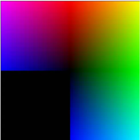
Fig. 1. Triple of the 2D histogram in RGB color space presented as three Euclidean graphs with two adjacent common axes

Although it is not a common practice, a 2D histogram can be presented with a background of histogram colors. The advantage of such presentation for RGB histograms is that apart from the point R=G=B=0 there is no other gray scale point in the histogram making the gray scale an ideal representative for the other important parameter of a histogram, the pixel count. Fig. 1 shows an example of such a background for the triple of 2D histograms of the RGB color space using the Euclidean approach to the histogram presentation. In the graph each of the three squares has 256×256 colors corresponding to all possible combinations of two components with the third components set to 0. Note that even if the three color maps are positioned so that two pairs of them RB and RG, RG and BG share a common axis, the third one is represented twice, separated by a large unused area. In this paper we consider a method and layout

Method of Visualization of Two-Dimensional

Histogram Set of a Color Image

Alexander A. Gutenev

of plotting such three histograms so that each axis is plotted only once giving in our opinion a better perception of the relationships between the histograms in the triple.

II. PROPOSED LAYOUT OF THE 2D HISTOGRAM TRIPLE

A. Segmenting of a tiled surface onto three adjacent areas each made of lines parallel to two axes

A standard digital image consists of square pixels. The sides of the pixels are aligned with the sides of the image. The image plane can be considered tiled with such pixels. Let us consider the geometry of the lines consisting of such square pixels.

Definition: A tiled line is a set of tiles (pixels) where each tile of the line apart from two tiles called end points has two and only two adjacent or neighbor tiles belonging to the line. A tiled line is a line one pixel in thickness.

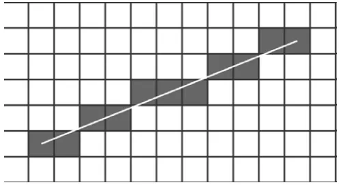
Consider a tiled line approximating a continuous line on a plane given by the equation Y= a × X + b, where X is the horizontal and Y is the vertical axes of the image, a is the slope, b is the intercept. The tiled line can be constructed using Bresenham’s algorithm [4]. It can be considered as a sequence of horizontal or vertical segments. The direction of the segments depends on the slope. There are two special cases: a = π/4± π and a = 3π/4± π when each segment is one pixel long.

Fig. 2. A tiled line approximating a straight line

If –π/4 < tan-1_{(a) < π/4, then the tiled line does not have a} single vertical segment higher than one pixel, that is xi ≠ xi+1, if yi=yi+1 ± 1. Accordingly, if π/4 < tan-1_{(a) < 3π/4, then} the tiled line does not have a single horizontal segment higher than one pixel, that is yi ≠ yi+1, if xi=xi+1 ± 1.

Parallel tiled lines are generated from a single line by shifting all its pixels by n tiles in X direction and m tiles in Y direction, where n and m are arbitrary integer numbers.

Consider an image plane covered densely and without overlap with parallel lines.

Theorem 1. Tiling of the plane with parallel digital lines can only be performed if the lines run parallel to the pixel edges or at π/4± π or 3π/4± π to the edges.

Proof: Two digital lines are parallel, if one of them is a replica of the other, shifted within the digital plane by n units in horizontal direction (X) and m units in vertical

direction (Y), where n and m are arbitrary integer numbers. Consider a base line which is not parallel to the axis X or Y and not running at π/4± π or 3π/4± π to either of them. Such a line will always have at least one segment consisting of at least two pixels parallel to the horizontal or vertical axis. For the sake of certainty let us assume that this segment is parallel to the horizontal axis. Then there exists a horizontal shift by one pixel such that the shifted line will intersect with the base line. On the other hand, if the tiled line consists of the segments one pixel long and one pixel wide, any shift by any number of pixels in any direction apart from along the line will produce a line parallel to the base line.

Theorem 2: Splitting the plane into three areas tiled by parallel tile lines can only be performed if two axes are orthogonal to each other and the third one is at the angle 3π/4 with respect to both of them.

The proof is an obvious result of the Theorem 1. Since the tiling by the parallel lines can be performed only in the directions kπ/4, where k=0, ±1, ±2,…, two of the three axes have to be at the angle π/2 with respect to each other. This leaves the remaining axis the task of splitting the remaining 3π/2 into two parts. Fig. 3 shows an example of the axes layout.

Fig. 3. One of the configurations for axis layouts where three areas share common axes

B. Proposed Axis Layout

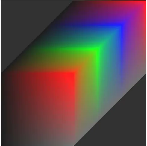
left, red axis going from the centre at 45o _{and the green axis} going from the centre down. Although the axes of the two areas of the map are not orthogonal, the underlying bitmaps of the 2D histogram colors indicate distinctively the color value in each point. The commonality of axes provides harmonious transition from the area of one histogram to the area of another.

Fig. 4. One of possible layouts maintaining axis adjacency

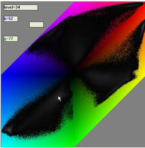
Fig. 5. RGB 2D histogram triple for the Baboon image. The cursor points to the Blue-Green part, where blue =52, green = 72 and the pixel count is 34

III. EXAMPLES AND ANALYSIS

A. Application of the Proposed Layout in the Interactive Environment

The continuous nature of the background map shown in Fig. 4 removes the need for markings on the axes assuming that there are other ways of showing the value pairs for the 2D histogram. Those markings placed on the axes normally would obscure the data due to the proximity of the histogram areas. From this point of view, the layout is better suited to an interactive environment: when the actual values are required, they are displayed as the user moves the cursor over the area. Fig. 5 shows an example of a histogram triple for the standard image “baboon” Fig. 6. Fig. 5 represents one of the ways of displaying the value pairs and the pixel count for that pair. This histogram is presented as a map of gray pixels for the pixels present in the image and colored pixels for the ones missing in the image. The pixel count for each participating pair is shown by a gray level with intensity increasing with the count. The color corresponds to the 2 color components with the third component having a fixed value. In the cases of Fig. 4 and Fig. 5 the fixed value is 0.

The implementation of the 2D histograms described above is available as part of the Pictorial Image Processor© package at www.pic-i-proc.com.

Fig. 6. Image from a standard dataset producing 2D histogram triple Fig. 5

B. Application with Various Color Spaces

black. For such color spaces it is better to place the point of maximum intensity into the origin and decrement the intensity towards the edge of the graph. The RGB color space (Fig. 4) does not have an explicit intensity component, hence the position of the minimum intensity point in the graph’s origin. The same applies to the complimentary cyan-magenta-yellow (CMY) color space. Fig. 7 shows the use of this layout with the CMY color space. The transition lines between the 2D histograms appear quite natural.

The color spaces with circular components like hue-saturation-intensity (HSI) are much harder to interpret using this layout. It has a distinct intensity component; hence the origin of the graph should have this component at a maximum. The saturation component should also be maximal in the origin. Otherwise the saturation-hue panel becomes just shades of gray since at zero saturation all color is lost. The origin and direction of the hue component are non-essential since the component is circular, starting and finishing at the color red.

Fig. 7. Use of the proposed layout with CMY color space

Fig. 8 shows the map for HSI color space with the intensity axis going horizontally from the left to the centre of the graph, saturation axis going from the bottom up to the centre and the hue axis going from the corner at 45o _towards the centre.

One can see that at low intensity all colors collapse to black and that at high saturation they all wash out into shades of gray. Due to the high number of low intensity and low saturation pixels, the average intensity of the map Fig. 8 without additional brightening would have been quite low. In order to improve the visibility of the map, its intensity was increased by 12% with respect to the calculated values.

Fig. 8. Use of the proposed layout with the HSI color space

Note the black lines limiting the graph on the left. They represent zero intensity. The gray line at 45o _{on the right} represents maximum intensity and zero saturation. The presence of a significant number of grey pixels in the background image introduces an additional challenge to the presentation of the pixel counts in such a 2D histogram. One can still use shades of gray to represent pixel counts as in Fig. 5, but there is a risk that some of the pixel counts will not be distinguishable from the background.

Fig. 9 shows the proposed presentation of the HSI histogram triple for the standard image Fig.5.

REFERENCES

[1] O. Lezoray, An unsupervised color image segmentation based on morphological 2D clustering and fusion, in Color in Graphics, Imaging and Vision, CGIV, 2004 , pp. 173-177.

[2] Meng Fan-jie, Guo Bao-long, Guo Lei, “ Image Retrieval Based on 2D Histogram of Interest Points,” in Fifth International Conference on Information Assurance and Security, 2009. IAS '09, pp. 250 – 253. [3] A. Hanbury, B. Marcotegui, “Colour Adjacency Histograms for Image

Matching,” in CAIP'07 Proceedings of the 12th international conference on Computer analysis of images and patterns, Berlin: Springer-Verlag, 2007 pp 424-431

[4] Jack E. Bresenham, "Algorithm for computer control of a digital plotter", IBM Systems Journal, Vol. 4, No.1, January 1965, pp. 25–30 [5] Hsien-Che Lee, Introduction to Color Imaging Science. Cambridge

University Press, 2009

[6] E. Reinhard , E. A. Khan , A. O. Akyüz , Garrett M. Johnson, Color Imaging: Fundamentals and Applications. A.K. Peters Ltd Wellesley, MA, 2008